We start from a large data-set $V=\{ k,l,m,n,\dots \}$ (texts, events, DNA-samples, …) with a suitable distance-function ($d(m,n) \geq 0~d(k,l)+d(l,m) \geq d(k.m)$) which measures the (dis)similarity between individual samples.
We’re after a set of unknown events $\{ p,q,r,s,\dots \}$ to explain the distances between the observed data. An example: let’s assume we’ve sequenced the DNA of a set of species, and computed a Hamming-like distance to measures the differences between these sequences.
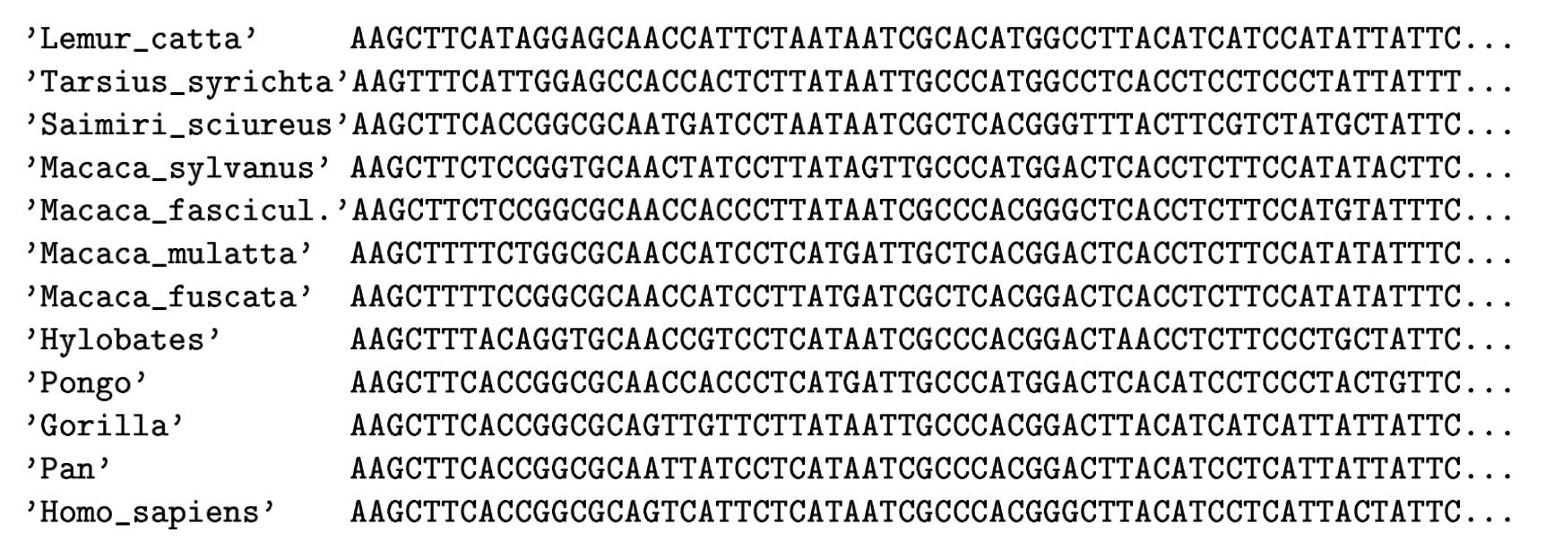
(From Geometry of the space of phylogenetic trees by Billera, Holmes and Vogtmann)
Biology explains these differences from the fact that certain species may have had more recent common ancestors than others. Ideally, the measured distances between DNA-samples are a tree metric. That is, if we can determine the full ancestor-tree of these species, there should be numbers between ancestor-nodes (measuring their difference in DNA) such that the distance between two existing species is the sum of distances over the edges of the unique path in this phylogenetic tree connecting the two species.
Last time we’ve see that a necessary and sufficient condition for a tree-metric is that for every quadruple $k,l,m,n \in V$ we have that the maximum of the sum-distances
$$\{ d(k,l)+d(m,n),~d(k,m)+d(l,n),~d(k,n)+d(l,m) \}$$
is attained at least twice.
In practice, it rarely happens that the measured distances between DNA-samples are a perfect fit to this condition, but still we would like to compute the most probable phylogenetic tree. In the above example, there will be two such likely trees:
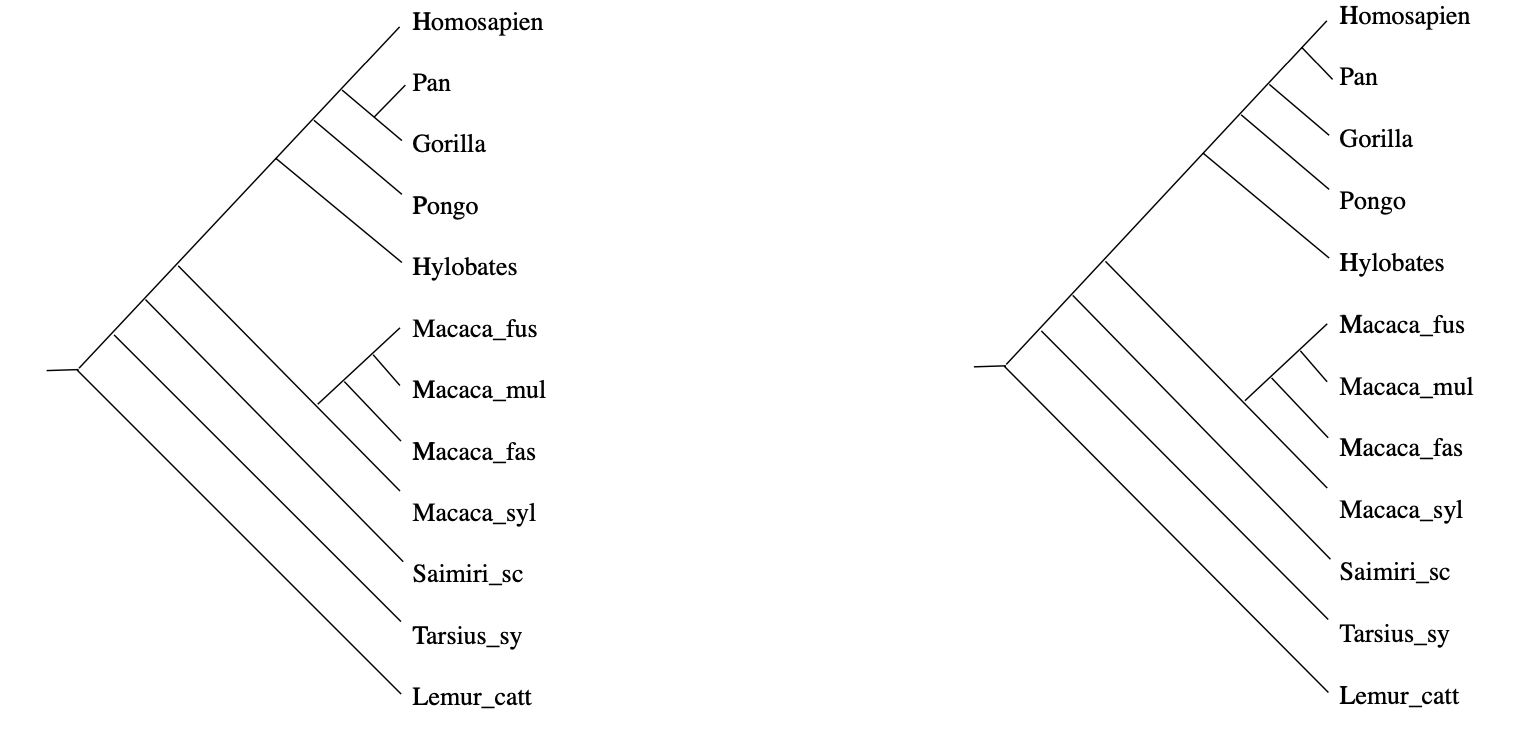
(From Geometry of the space of phylogenetic trees by Billera, Holmes and Vogtmann)
How can we find them? And, if the distances in our data-set do not have such a direct biological explanation, is it still possible to find such trees of events (or perhaps, a forest of event-trees) explaining our distance function?
Well, tracking back these ancestor nodes looks a lot like trying to construct colimits.
By now, every child knows that if their toy category $T$ does not allow them to construct all colimits, they can always beg for an upgrade to the presheaf topos $\widehat{T}$ of all contravariant functors from $T$ to $Sets$.
But then, the child can cobble together too many crazy constructions, and the parents have to call in the Grothendieck police who will impose one of their topologies to keep things under control.
Can we fall back on this standard topos philosophy in order to find these forests of the unconscious?
(Image credit)
We have a data-set $V$ with a distance function $d$, and it is fashionable to call this setting a $[0,\infty]$-‘enriched’ category. This is a misnomer, there’s not much ‘category’ in a $[0,\infty]$-enriched category. The only way to define an underlying category from it is to turn $V$ into a poset via $n \geq m$ iff $d(n,m)=0$.
Still, we can define the set $\widehat{V}$ of $[0,\infty]$-enriched presheaves, consisting of all maps
$$p : V \rightarrow [0,\infty] \quad \text{satisfying} \quad \forall m,n \in V : d(m,n)+p(n) \geq p(m)$$
which is again a $[0,\infty]$-enriched category with distance function
$$\hat{d}(p,q) = \underset{m \in V}{max} (q(m) \overset{.}{-} p(m)) \quad \text{with} \quad a \overset{.}{-} b = max(a-b,0)$$
so $\widehat{V}$ is a poset via $p \geq q$ iff $\forall m \in V : p(m) \geq q(m)$.
The good news is that $\widehat{V}$ contains all limits and colimits (because $[0,\infty]$ has sup’s and inf’s) and that $V$ embeds isometrically in $\widehat{V}$ via the Yoneda-map
$$m \mapsto y_m \quad \text{with} \quad y_m(n)=d(n,m)$$
The mental picture of a $[0,\infty]$-enriched presheaf $p$ is that of an additional ‘point’ with $p(m)$ the distance from $y_m$ to $p$.
But there’s hardly a subobject classifier to speak of, and so no Grothendieck topologies nor internal logic. So, how can we select from the abundance of enriched presheaves, the nodes of our event-forest?
We can look for special properties of the ancestor-nodes in a phylogenetic tree.
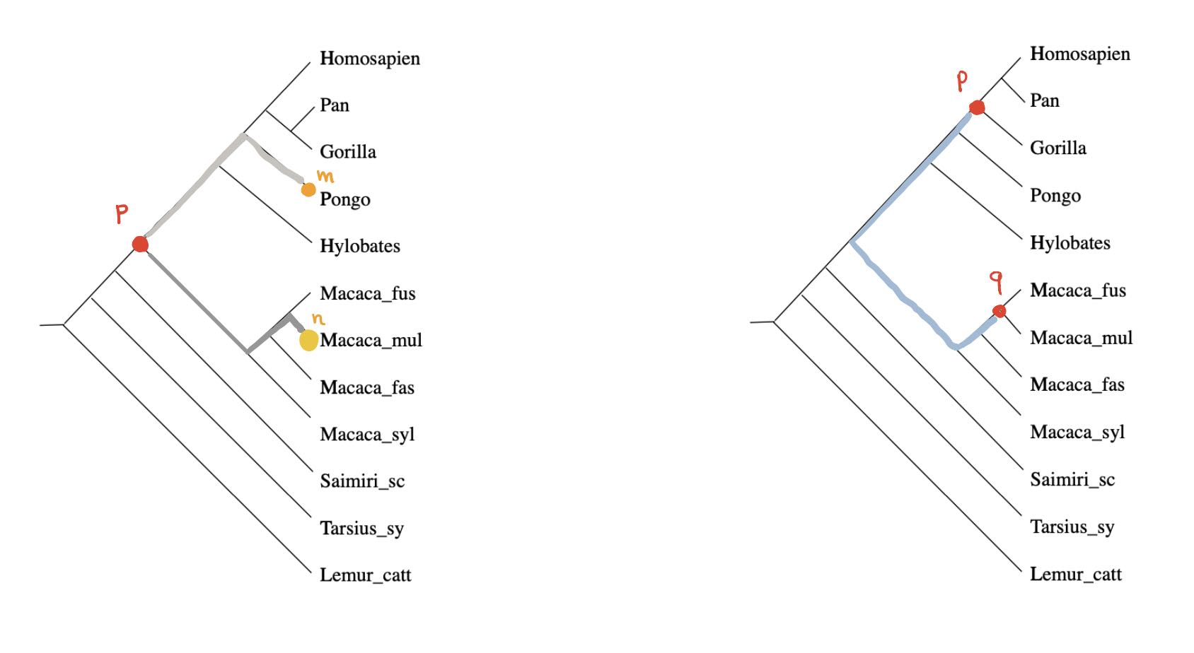
For any ancestor node $p$ and any $m \in V$ there is a unique branch from $p$ having $m$ as a leaf (picture above,left). Take another branch in $p$ and a leaf vertex $n$ of it, then the combination of these two paths gives the unique path from $m$ to $n$ in the phylogenetic tree, and therefore
$$\hat{d}(y_m,y_n) = d(m,n) = p(m)+p(n) = \hat{d}(p,y_m) + \hat{d}(p,y_n)$$
In other words, for every $m \in V$ there is another $n \in V$ such that $p$ lies on the geodesic from $m$ to $n$ (identifying elements of $V$ with their Yoneda images in $\widehat{V}$).
Compare this to Stephen Wolfram’s belief that if we looked properly at “what ChatGPT is doing inside, we’d immediately see that ChatGPT is doing something “mathematical-physics-simple” like following geodesics”.
Even if the distance on $V$ is symmetric, the extended distance function on $\widehat{V}$ is usually far from symmetric. But here, as we’re dealing with a tree-distance, we have for all ancestor-nodes $p$ and $q$ that $\hat{d}(p,q)=\hat{d}(q,p)$ as this is just the sum of the weights of the edges on the unique path from $p$ and $q$ (picture above, on the right).
Right, now let’s look at a non-tree distance function on $V$, and let’s look at those elements in $\widehat{V}$ having similar properties as the ancestor-nodes:
$$T_V = \{ p \in \widehat{V}~:~\forall n \in V~:~p(n) = \underset{m \in V}{max} (d(m,n) \overset{.}{-} p(m)) \}$$
Then again, for every $p \in T_V$ and every $n \in V$ there is an $m \in V$ such that $p$ lies on a geodesic from $n$ to $m$.
The simplest non-tree example is $V = \{ a,b,c,d \}$ with say
$$d(a,c)+d(b,d) > max(d(a,b)+d(c,d),d(a,d)+d(b,c))$$
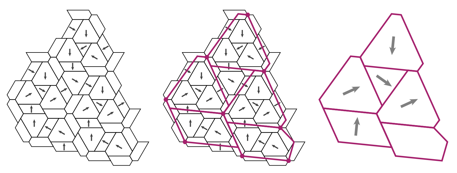
In this case, $T_V$ was calculated by Andreas Dress in Trees, Tight Extensions of Metric Spaces, and the Cohomological Dimension of Certain Groups: A Note on Combinatorial Properties of Metric Spaces. Note that Dress writes $mn$ for $d(m,n)$.
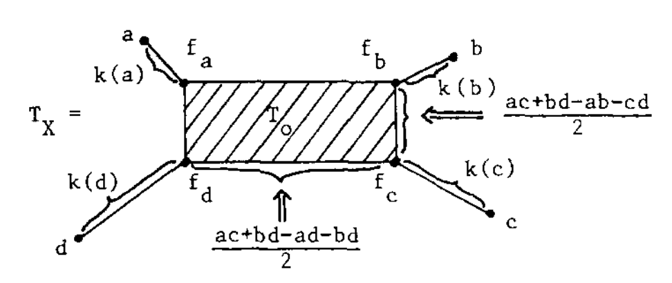
If this were a tree-metric, $T_V$ would be the tree, but now we have a $2$-dimensional cell $T_0$ consisting of those presheaves lying on a geodesic between $a$ and $c$, and on the one between $b$ and $d$. Let’s denote this by $T_0 = \{ a—c,b—d \}$.
$T_V$ has eight $1$-dimensional cells, and with the same notation we have
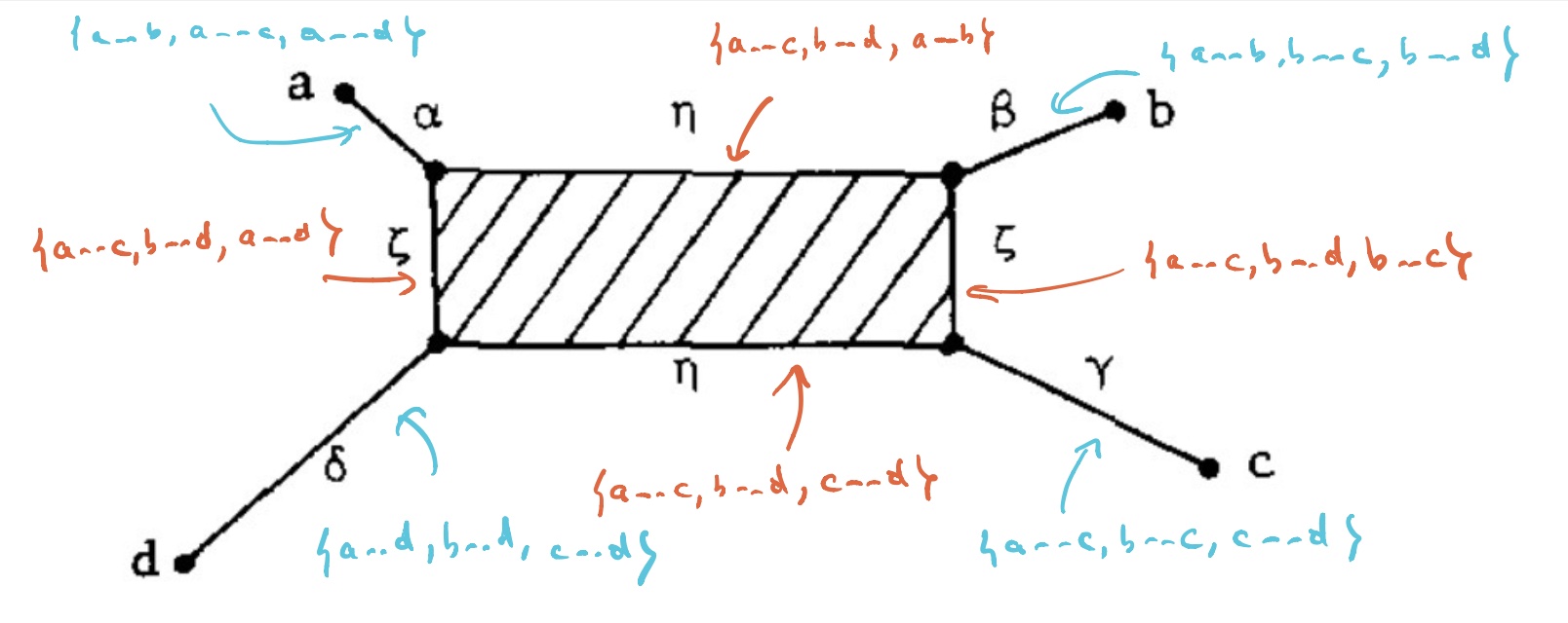
Let’s say that $V= \{ a,b,c,d \}$ are four DNA-samples of species but failed to satisfy the tree-metric condition by an error in the measurements, how can we determine likely phylogenetic trees for them? Well, given the shape of the cell-complex $T_V$ there are four spanning trees (with root in $f_a,f_b,f_c$ or $f_d$) having the elements of $V$ as their only leaf-nodes. Which of these is most likely the ancestor-tree will depend on the precise distances.
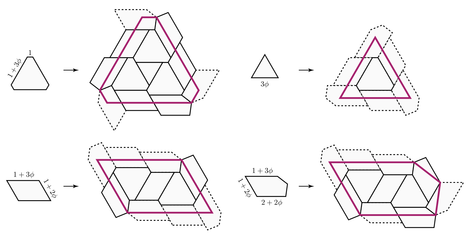
For an arbitrary data-set $V$, the structure of $T_V$ has been studied extensively, under a variety of names such as ‘Isbell’s injective hull’, ‘tight span’ or ‘tropical convex hull’, in slightly different settings. So, in order to use results one sometimes have to intersect with some (un)bounded polyhedron.
It is known that $T_V$ is always a cell-complex with dimension of the largest cell bounded by half the number of elements of $V$. In this generality it will no longer be the case that there is a rooted spanning tree of teh complex having the elements of $V$ as its only leaves, but we can opt for the best forest of rooted trees in the $1$-skeleton having all of $V$ as their leaf-nodes. Theses are the ‘forests of the unconscious’ explaining the distance function on the data-set $V$.
Apart from the Dress-paper mentioned above, I’ve found these papers informative:
- Metric spaces in pure and applied mathematics by Dress, Huber and Moulton
- Computing the bounded subcomplex of an unbounded polyhedron by Hermann, Joswig and Pfetsch
- Tropical convexity by Develin and Sturmfels
- Tight spans, Isbell completions and semi-tropical modules by Willerton
So far, we started from a data-set $V$ with a symmetric distance function, but for applications in LLMs one might want to drop that condition. In that case, Willerton proved that there is a suitable replacement of $T_V$, which is now called the ‘directed tight span’ and which coincides with the Isbell completion.
Recently, Simon Willerton gave a talk at the African Mathematical Seminar called ‘Looking at metric spaces as enriched categories’:
Willerton also posts a series(?) on this at the n-category cafe, starting with Metric spaces as enriched categories I.
(tbc?)
Previously in this series:
- The topology of dreams
- The shape of languages
- Loading a second brain
- The enriched vault
- The super-vault of missing notes
- The tropical brain-forest