Category: math

Sylvester’s synthemes

Published March 19, 2020 by lieven

I was running a bachelor course on representations of finite groups and a master course on simple (mainly sporadic) groups until Corona closed us down. Perhaps these blog-posts can be useful to some.

A curious fact, with ripple effect on Mathieu sporadic groups, is that the symmetric group $S_6$ has an automorphism $\phi$, different from an automorphism by conjugation.

In the course notes the standard approach was given, based on the $5$-Sylow subgroups of $S_5$.

Here’s the idea. Let $S_6$ act by permuting $6$ elements and consider the subgroup $S_5$ fixing say $6$. If such an odd automorphism $\phi$ would exist, then the subgroup $\phi(S_5)$ cannot fix one of the six elements (for then it would be conjugated to $S_5$), so it must act transitively on the six elements.

The alternating group $A_5$ is the rotation symmetry group of the icosahedron

Any $5$-Sylow subgroup of $A_5$ is the cyclic group $C_5$ generated by a rotation among one of the six body-diagonals of the icosahedron. As $A_5$ is normal in $S_5$, also $S_5$ has six $5$-Sylows.

More lowbrow, such a subgroup is generated by a permutation of the form $(1,2,a,b,c)$, of which there are six. Good old Sylow tells us that these $5$-Sylow subgroups are conjugated, giving a monomorphism
\[
S_5 \rightarrow Sym(\{ 5-Sylows \})\simeq S_6 \]
and its image $H$ is a subgroup of $S_6$ of index $6$ (and isomorphic to $S_5$) which acts transitively on six elements.

Left multiplication gives an action of $S_6$ on the six cosets $S_6/H =\{ \sigma H~:~\sigma \in S_6 \}$, that is a groupmorphism
\[
\phi : S_6 \rightarrow Sym(\{ \sigma H \}) = S_6 \]
which is our odd automorphism (actually it is even, of order two). A calculation shows that $\phi$ sends permutations of cycle shape $2.1^4$ to shape $2^3$, so can’t be given by conjugation (which preserves cycle shapes).

An alternative approach is given by Noah Snyder in an old post at the Secret Blogging Seminar.

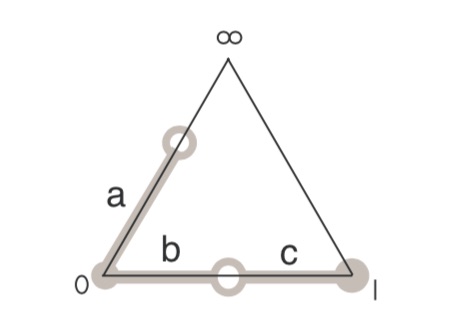
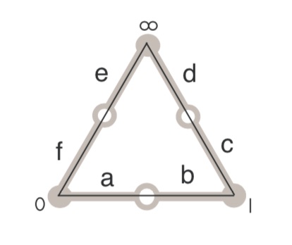
Here, we like to identify the six points $\{ a,b,c,d,e,f \}$ with the six points $\{ 0,1,2,3,4,\infty \}$ of the projective line $\mathbb{P}^1(\mathbb{F}_5)$ over the finite field $\mathbb{F}_5$.

There are $6!$ different ways to do this set-theoretically, but lots of them are the same up to an automorphism of $\mathbb{P}^1(\mathbb{F}_5)$, that is an element of $PGL_2(\mathbb{F}_5)$ acting via Mobius transformations on $\mathbb{P}^1(\mathbb{F}_5)$.

$PGL_2(\mathbb{F}_5)$ acts $3$-transitively on $\mathbb{P}^1(\mathbb{F}_5)$ so we can fix three elements in each class, say $a=0,b=1$ and $f=\infty$, leaving six different ways to label the points of the projective line
\[
\begin{array}{c|cccccc}
& a & b & c & d & e & f \\
\hline
1 & 0 & 1 & 2 & 3 & 4 & \infty \\
2 & 0 & 1 & 2 & 4 & 3 & \infty \\
3 & 0 & 1 & 3 & 2 & 4 & \infty \\
4 & 0 & 1 & 3 & 4 & 2 & \infty \\
5 & 0 & 1 & 4 & 2 & 3 & \infty \\
6 & 0 & 1 & 4 & 3 & 2 & \infty
\end{array}
\]
A permutation of the six elements $\{ a,b,c,d,e,f \}$ will result in a permutation of the six classes of $\mathbb{P}^1(\mathbb{F}_5)$-labelings giving the odd automorphism
\[
\phi : S_6 = Sym(\{ a,b,c,d,e,f \}) \rightarrow Sym(\{ 1,2,3,4,5,6 \}) = S_6 \]
An example: the involution $(a,b)$ swaps the points $0$ and $1$ in $\mathbb{P}^1(\mathbb{F}_5)$, which can be corrected via the Mobius-automorphism $t \mapsto 1-t$. But this automorphism has an effect on the remaining points
\[
2 \leftrightarrow 4 \qquad 3 \leftrightarrow 3 \qquad \infty \leftrightarrow \infty \]
So the six different $\mathbb{P}^1(\mathbb{F}_5)$ labelings are permuted as
\[
\phi((a,b))=(1,6)(2,5)(3,4) \]
showing (again) that $\phi$ is not a conjugation-automorphism.

Yet another, and in fact the original, approach by James Sylvester uses the strange terminology of duads, synthemes and synthematic totals.

A duad is a $2$-element subset of $\{ 1,2,3,4,5,6 \}$ (there are $15$ of them).
A syntheme is a partition of $\{ 1,2,3,4,5,6 \}$ into three duads (there are $15$ of them).
A (synthematic) total is a partition of the $15$ duads into $5$ synthemes, and they are harder to count.

There’s a nice blog-post by Peter Cameron on this, as well as his paper From $M_{12}$ to $M_{24}$ (after Graham Higman). As my master-students have to work their own way through this paper I will not spoil their fun in trying to deduce that

Two totals have exactly one syntheme in common, so synthemes are ‘duads of totals’.
Three synthemes lying in disjoint pairs of totals must consist of synthemes containing a fixed duad, so duads are ‘synthemes of totals’.
Duads come from disjoint synthemes of totals in this way if and only if they share a point, so points are ‘totals of totals’

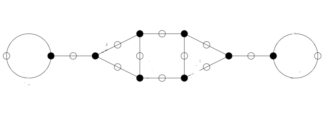
My hint to the students was “Google for John Baez+six”, hoping they’ll discover Baez’ marvellous post Some thoughts on the number $6$, and in particular, the image (due to Greg Egan) in that post

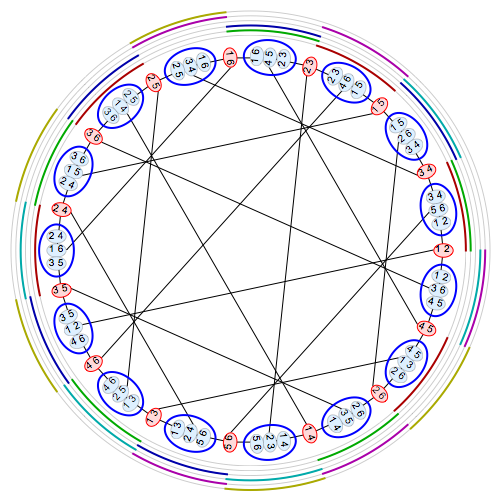
which makes everything visually clear.

The duads are the $15$ red vertices, the synthemes the $15$ blue vertices, connected by edges when a duad is contained in a syntheme. One obtains the Tutte-Coxeter graph.

The $6$ concentric rings around the picture are the $6$ synthematic totals. A band of color appears in one of these rings near some syntheme if that syntheme is part of that synthematic total.

If $\{ t_1,t_2,t_3,t_4,t_5,t_6 \}$ are the six totals, then any permutation $\sigma$ of $\{ 1,2,3,4,5,6 \}$ induces a permutation $\phi(\sigma)$ of the totals, giving the odd automorphism
\[
\phi : S_6 = Sym(\{ 1,2,3,4,5,6 \}) \rightarrow Sym(\{ t_1,t_2,t_3,t_4,t_5,t_6 \}) = S_6 \]

Comments closed

Dessinflateurs

Published August 10, 2019 by lieven

I’m trying to get into the latest Manin-Marcolli paper Quantum Statistical Mechanics of the Absolute Galois Group on how to create from Grothendieck’s dessins d’enfant a quantum system, generalising the Bost-Connes system to the non-Abelian part of the absolute Galois group $Gal(\overline{\mathbb{Q}}/\mathbb{Q})$.

In doing so they want to extend the action of the multiplicative monoid $\mathbb{N}_{\times}$ by power maps on the roots of unity to the action of a larger monoid on all dessins d’enfants.

Here they use an idea, originally due to Jordan Ellenberg, worked out by Melanie Wood in her paper Belyi-extending maps and the Galois action on dessins d’enfants.

To grasp this, it’s best to remember what dessins have to do with Belyi maps, which are maps defined over $\overline{\mathbb{Q}}$
\[
\pi : \Sigma \rightarrow \mathbb{P}^1 \]
from a Riemann surface $\Sigma$ to the complex projective line (aka the 2-sphere), ramified only in $0,1$ and $\infty$. The dessin determining $\pi$ is the 2-coloured graph on the surface $\Sigma$ with as black vertices the pre-images of $0$, white vertices the pre-images of $1$ and these vertices are joined by the lifts of the closed interval $[0,1]$, so the number of edges is equal to the degree $d$ of the map.

Wood considers a very special subclass of these maps, which she calls Belyi-extender maps, of the form
\[
\gamma : \mathbb{P}^1 \rightarrow \mathbb{P}^1 \]
defined over $\mathbb{Q}$ with the additional property that $\gamma$ maps $\{ 0,1,\infty \}$ into $\{ 0,1,\infty \}$.

The upshot being that post-compositions of Belyi’s with Belyi-extenders $\gamma \circ \pi$ are again Belyi maps, and if two Belyi’s $\pi$ and $\pi’$ lie in the same Galois orbit, then so must all $\gamma \circ \pi$ and $\gamma \circ \pi’$.

The crucial Ellenberg-Wood idea is then to construct “new Galois invariants” of dessins by checking existing and easily computable Galois invariants on the dessins of the Belyi’s $\gamma \circ \pi$.

For this we need to know how to draw the dessin of $\gamma \circ \pi$ on $\Sigma$ if we know the dessins of $\pi$ and of the Belyi-extender $\gamma$. Here’s the procedure

Here, the middle dessin is that of the Belyi-extender $\gamma$ (which in this case is the power map $t \rightarrow t^4$) and the upper graph is the unmarked dessin of $\pi$.

One has to replace each of the black-white edges in the dessin of $\pi$ by the dessin of the expander $\gamma$, but one must be very careful in respecting the orientations on the two dessins. In the upper picture just one edge is replaced and one has to do this for all edges in a compatible manner.

Thus, a Belyi-expander $\gamma$ inflates the dessin $\pi$ with factor the degree of $\gamma$. For this reason i prefer to call them dessinflateurs, a contraction of dessin+inflator.

In her paper, Melanie Wood says she can separate dessins for which all known Galois invariants were the same, such as these two dessins,

by inflating them with a suitable Belyi-extender and computing the monodromy group of the inflated dessin.

This monodromy group is the permutation group generated by two elements, the first one gives the permutation on the edges given by walking counter-clockwise around all black vertices, the second by walking around all white vertices.

For example, by labelling the edges of $\Delta$, its monodromy is generated by the permutations $(2,3,5,4)(1,6)(8,10,9)$ and $(1,3,2)(4,7,5,8)(9,10)$ and GAP tells us that the order of this group is $1814400$. For $\Omega$ the generating permutations are $(1,2)(3,6,4,7)(8,9,10)$ and $(1,2,4,3)(5,6)(7,9,8)$, giving an isomorphic group.

Let’s inflate these dessins using the Belyi-extender $\gamma(t) = -\frac{27}{4}(t^3-t^2)$ with corresponding dessin

It took me a couple of attempts before I got the inflated dessins correct (as i knew from Wood that this simple extender would not separate the dessins). Inflated $\Omega$ on top:

Both dessins give a monodromy group of order $35838544379904000000$.

Now we’re ready to do serious work.

Melanie Wood uses in her paper the extender $\zeta(t)=\frac{27 t^2(t-1)^2}{4(t^2-t+1)^3}$ with associated dessin

and says she can now separate the inflated dessins by the order of their monodromy groups. She gets for the inflated $\Delta$ the order $19752284160000$ and for inflated $\Omega$ the order $214066877211724763979841536000000000000$.

It’s very easy to make mistakes in these computations, so probably I did something horribly wrong but I get for both $\Delta$ and $\Omega$ that the order of the monodromy group of the inflated dessin is $214066877211724763979841536000000000000$.

I’d be very happy when someone would be able to spot the error!

One Comment

Monstrous dessins 3

Published August 3, 2019 by lieven

A long while ago I promised to take you from the action by the modular group $\Gamma=PSL_2(\mathbb{Z})$ on the lattices at hyperdistance $n$ from the standard orthogonal laatice $L_1$ to the corresponding ‘monstrous’ Grothendieck dessin d’enfant.

Speaking of dessins d’enfant, let me point you to the latest intriguing paper by Yuri I. Manin and Matilde Marcolli, ArXived a few days ago Quantum Statistical Mechanics of the Absolute Galois Group, on how to build a quantum system for the absolute Galois group from dessins d’enfant (more on this, I promise, later).

Where were we?

We’ve seen natural one-to-one correspondences between (a) points on the projective line over $\mathbb{Z}/n\mathbb{Z}$, (b) lattices at hyperdistance $n$ from $L_1$, and (c) coset classes of the congruence subgroup $\Gamma_0(n)$ in $\Gamma$.

How to get from there to a dessin d’enfant?

The short answer is: it’s all in Ravi S. Kulkarni’s paper, “An arithmetic-geometric method in the study of the subgroups of the modular group”, Amer. J. Math 113 (1991) 1053-1135.

It is a complete mystery to me why Tatitscheff, He and McKay don’t mention Kulkarni’s paper in “Cusps, congruence groups and monstrous dessins”. Because all they do (and much more) is in Kulkarni.

I’ve blogged about Kulkarni’s paper years ago:

– In the Dedekind tessalation it was all about assigning special polygons to subgroups of finite index of $\Gamma$.

– In Modular quilts and cuboid tree diagram it did go on assigning (multiple) cuboid trees to a (conjugacy class) of such finite index subgroup.

– In Hyperbolic Mathieu polygons the story continued on a finite-to-one connection between special hyperbolic polygons and cuboid trees.

– In Farey codes it was shown how to encode such polygons by a Farey-sequence.

– In Generators of modular subgroups it was shown how to get generators of the finite index subgroups from this Farey sequence.

The modular group is a free product
\[
\Gamma = C_2 \ast C_3 = \langle s,u~|~s^2=1=u^3 \rangle \]
with lifts of $s$ and $u$ to $SL_2(\mathbb{Z})$ given by the matrices
\[
S=\begin{bmatrix} 0 & -1 \\ 1 & 0 \end{bmatrix},~\qquad U= \begin{bmatrix} 0 & -1 \\ 1 & -1 \end{bmatrix} \]

As a result, any permutation representation of $\Gamma$ on a set $E$ can be represented by a $2$-coloured graph (with black and white vertices) and edges corresponding to the elements of the set $E$.

Each white vertex has two (or one) edges connected to it and every black vertex has three (or one). These edges are the elements of $E$ permuted by $s$ (for white vertices) and $u$ (for black ones), the order of the 3-cycle determined by going counterclockwise round the vertex.

Clearly, if there’s just one edge connected to a vertex, it gives a fixed point (or 1-cycle) in the corresponding permutation.

The ‘monstrous dessin’ for the congruence subgroup $\Gamma_0(n)$ is the picture one gets from the permutation $\Gamma$-action on the points of $\mathbb{P}^1(\mathbb{Z}/n \mathbb{Z})$, or equivalently, on the coset classes or on the lattices at hyperdistance $n$.

Kulkarni’s paper (or the blogposts above) tell you how to get at this picture starting from a fundamental domain of $\Gamma_0(n)$ acting on teh upper half-plane by Moebius transformations.

Sage gives a nice image of this fundamental domain via the command

FareySymbol(Gamma0(n)).fundamental_domain()

Here’s the image for $n=6$:

The boundary points (on the halflines through $0$ and $1$ and the $4$ half-circles need to be identified which is indicaed by matching colours. So the 2 halflines are identified as are the two blue (and green) half-circles (in opposite direction).

To get the dessin from this, let’s first look at the interior points. A white vertex is a point in the interior where two black and two white tiles meet, a black vertex corresponds to an interior points where three black and three white tiles meet.

Points on the boundary where tiles meet are coloured red, and after identification two of these reds give one white or black vertex. Here’s the intermediate picture

The two top red points are identified giving a white vertex as do the two reds on the blue half-circles and the two reds on the green half-circles, because after identification two black and two white tiles meet there.

This then gives us the ‘monstrous’ modular dessin for $n=6$ of the Tatitscheff, He and McKay paper:

Let’s try a more difficult example: $n=12$. Sage gives us as fundamental domain

giving us the intermediate picture

and spotting the correct identifications, this gives us the ‘monstrous’ dessin for $\Gamma_0(12)$ from the THM-paper:

In general there are several of these 2-coloured graphs giving the same permutation representation, so the obtained ‘monstrous dessin’ depends on the choice of fundamental domain.

You’ll have noticed that the domain for $\Gamma_0(6)$ was symmetric, whereas the one Sage provides for $\Gamma_0(12)$ is not.

This is caused by Sage using the Farey-code
\[
\xymatrix{
0 \ar@{-}[r]_1 & \frac{1}{6} \ar@{-}[r]_1 & \frac{1}{5} \ar@{-}[r]_2 & \frac{1}{4} \ar@{-}[r]_3 & \frac{1}{3} \ar@{-}[r]_4 & \frac{1}{2} \ar@{-}[r]_4 & \frac{2}{3} \ar@{-}[r]_3 & \frac{3}{4} \ar@{-}[r]_2 & 1}
\]

One of the nice results from Kulkarni’s paper is that for any $n$ there is a symmetric Farey-code, giving a perfectly symmetric fundamental domain for $\Gamma_0(n)$. For $n=12$ this symmetric code is

\[
\xymatrix{
0 \ar@{-}[r]_1 & \frac{1}{6} \ar@{-}[r]_2 & \frac{1}{4} \ar@{-}[r]_3 & \frac{1}{3} \ar@{-}[r]_4 & \frac{1}{2} \ar@{-}[r]_4 & \frac{2}{3} \ar@{-}[r]_3 & \frac{3}{4} \ar@{-}[r]_2 & \frac{5}{6} \ar@{-}[r]_1 & 1}
\]

It would be nice to see whether using these symmetric Farey-codes gives other ‘monstrous dessins’ than in the THM-paper.

Remains to identify the edges in the dessin with the lattices at hyperdistance $n$ from $L_1$.

Using the tricks from the previous post it is quite easy to check that for any $n$ the monstrous dessin for $\Gamma_0(n)$ starts off with the lattices $L_{M,\frac{g}{h}} = M,\frac{g}{h}$ as below

Let’s do a sample computation showing that the action of $s$ on $L_n$ gives $L_{\frac{1}{n}}$:

\[
L_n.s = \begin{bmatrix} n & 0 \\ 0 & 1 \end{bmatrix} \begin{bmatrix} 0 & -1 \\ 1 & 0 \end{bmatrix} = \begin{bmatrix} 0 & -n \\ 1 & 0 \end{bmatrix} \]

and then, as last time, to determine the class of the lattice spanned by the rows of this matrix we have to compute

\[
\begin{bmatrix} 0 & -1 \\ 1 & 0 \end{bmatrix} \begin{bmatrix} 0 & -n \\ 1 & 0 \end{bmatrix} = \begin{bmatrix} -1 & 0 \\ 0 & -n \end{bmatrix} \]

which is class $L_{\frac{1}{n}}$. And similarly for the other edges.

2 Comments