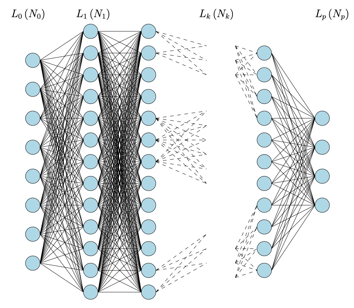
Brendan Fong, David Spivak and Remy Tuyeras cooked up a vast generalisation of neural networks in their paper Backprop as Functor: A compositional perspective on supervised learning.
Here’s a nice introduction to neural networks for category theorists by Bruno Gavranovic. At 1.49m he tries to explain supervised learning with neural networks in one slide. Learners show up later in the talk.
$\mathbf{Poly}$ is the category of all polynomial functors, that is, things of the form
\[
p = \sum_{i \in p(1)} y^{p[i]}~:~\mathbf{Sets} \rightarrow \mathbf{Sets} \qquad S \mapsto \bigsqcup_{i \in p(1)} Maps(p[i],S) \]
with $p(1)$ and all $p[i]$ sets.
Last time I gave Spivak’s ‘corolla’ picture to think about such functors.
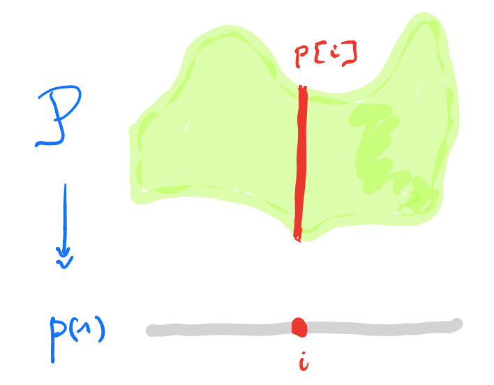
I prefer to view $p \in \mathbf{Poly}$ as an horribly discrete ‘sheaf’ $\mathcal{P}$ over the ‘space’ $p(1)$ with stalk $p[i]=\mathcal{P}_i$ at point $i \in p(1)$.
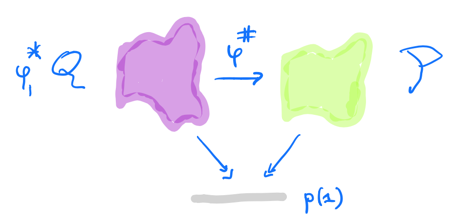
A morphism $p \rightarrow q$ in $\mathbf{Poly}$ is a map $\varphi_1 : p(1) \rightarrow q(1)$, together with for all $i \in p(1)$ a map $\varphi^{\#}_i : q[\varphi_1(i)] \rightarrow p[i]$.
In the sheaf picture, this gives a map of sheaves over the space $p(1)$ from the inverse image sheaf $\varphi_1^* \mathcal{Q}$ to $\mathcal{P}$.
But, unless you dream of sheaves in the night, by all means stick to Spivak’s corolla picture.
A learner $A \rightarrow B$ between two sets $A$ and $B$ is a complicated tuple of things $(P,I,U,R)$:
- $P$ is a set, a parameter space of some maps from $A$ to $B$.
- $I$ is the interpretation map $I : P \times A \rightarrow B$ describing the maps in $P$.
- $U$ is the update map $U : P \times A \times B \rightarrow P$, the learning procedure. The idea is that $U(p,a,b)$ is a map which sends $a$ closer to $b$ than the map $p$ did.
- $R$ is the request map $R : P \times A \times B \rightarrow A$.
Here’s a nice application of $\mathbf{Poly}$’s set-up:
Morphisms $\mathbf{P y^P \rightarrow Maps(A,B) \times Maps(A \times B,A) y^{A \times B}}$ in $\mathbf{Poly}$ coincide with learners $\mathbf{A \rightarrow B}$ with parameter space $\mathbf{P}$.
This follows from unpacking the definition of morphism in $\mathbf{Poly}$ and the process CT-ers prefer to call Currying.
The space-map $\varphi_1 : P \rightarrow Maps(A,B) \times Maps(A \times B,A)$ gives us the interpretation and request-map, whereas the sheaf-map $\varphi^{\#}$ gives us the more mysterious update-map $P \times A \times B \rightarrow P$.
$\mathbf{Learn(A,B)}$ is the category with objects all the learners $A \rightarrow B$ (for all paramater-sets $P$), and with morphisms defined naturally, that is, maps between the parameter-sets, compatible with the structural maps.
A surprising result from David Spivak’s paper Learners’ Languages is
$\mathbf{Learn(A,B)}$ is a topos. In fact, it is the topos of all set-valued representations of a (huge) directed graph $\mathbf{G_{AB}}$.
This will take some time.
Let’s bring some dynamics in. Take any polynmial functor $p \in \mathbf{Poly}$ and fix a morphism in $\mathbf{Poly}$
\[
\varphi = (\varphi_1,\varphi[-])~:~p(1) y^{p(1)} \rightarrow p \]
with space-map $\varphi_1$ the identity map.
We form a directed graph:
- the vertices are the elements of $p(1)$,
- vertex $i \in p(1)$ is the source vertex of exactly one arrow for every $a \in p[i]$,
- the target vertex of that arrow is the vertex $\phi[i](a) \in p(1)$.
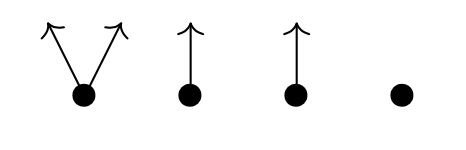
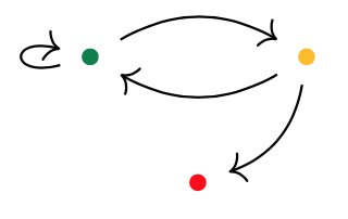
Here’s one possibility from Spivak’s paper for $p = 2y^2 + 1$, with the coefficient $2$-set $\{ \text{green dot, yellow dot} \}$, and with $1$ the singleton $\{ \text{red dot} \}$.
Start at one vertex and move after a minute along a directed edge to the next (possibly the same) vertex. The potential evolutions in time will then form a tree, with each node given a label in $p(1)$.
If we start at the green dot, we get this tree of potential time-evolutions
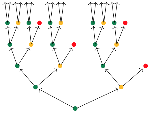
There are exactly $\# p[i]$ branches leaving a node labeled $i \in p(1)$, and all subtrees emanating from equal labelled nodes are isomorphic.
If we had started at the yellow dot we had obtained a labelled tree isomorphic to the subtree emanating here from any yellow dot.
We can do the same things for any morphism in $\mathbf{Poly}$ of the form
\[
\varphi = (\varphi_1,\varphi[-])~:~Sy^S \rightarrow p \]
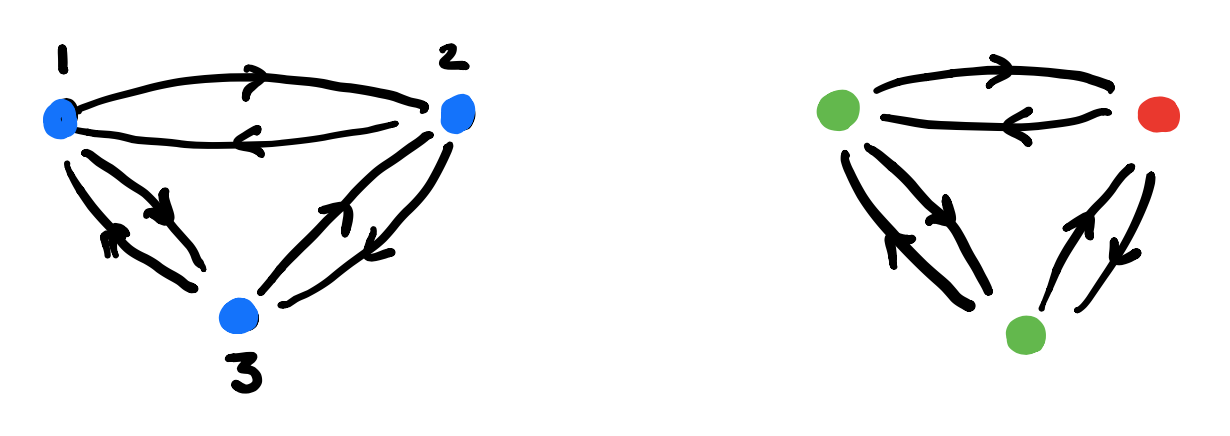
Now, we have a directed graph with vertices the elements $s \in S$, with as many edges leaving vertex $s$ as there are elements $a \in p[\varphi_1(s)]$, and with the target vertex of the edge labeled $a$ starting in $s$ the vertex $\varphi[\varphi_1(s)](A)$.
Once we have this directed graph on $\# S$ vertices we can label vertex $s$ with the label $\varphi_1(s)$ from $p(1)$.
In this way, the time evolutions starting at a vertex $s \in S$ will give us a $p(1)$-labelled rooted tree.
But now, it is possibly that two distinct vertices can have the same $p(1)$-labeled tree of evolutions. But also, trees corresponding to equal labeled vertices can be different.
Right, I guess we’re ready to define the graph $G_{AB}$ and prove that $\mathbf{Learn(A,B)}$ is a topos.
In the case of learners, we have the target polynomial functor $p=C y^{A \times B}$ with $C = Maps(A,B) \times Maps(A \times B,A)$, that is
\[
p(1) = C \quad \text{and all} \quad p[i]=A \times B \]
Start with the free rooted tree $T$ having exactly $\# A \times B$ branches growing from each node.
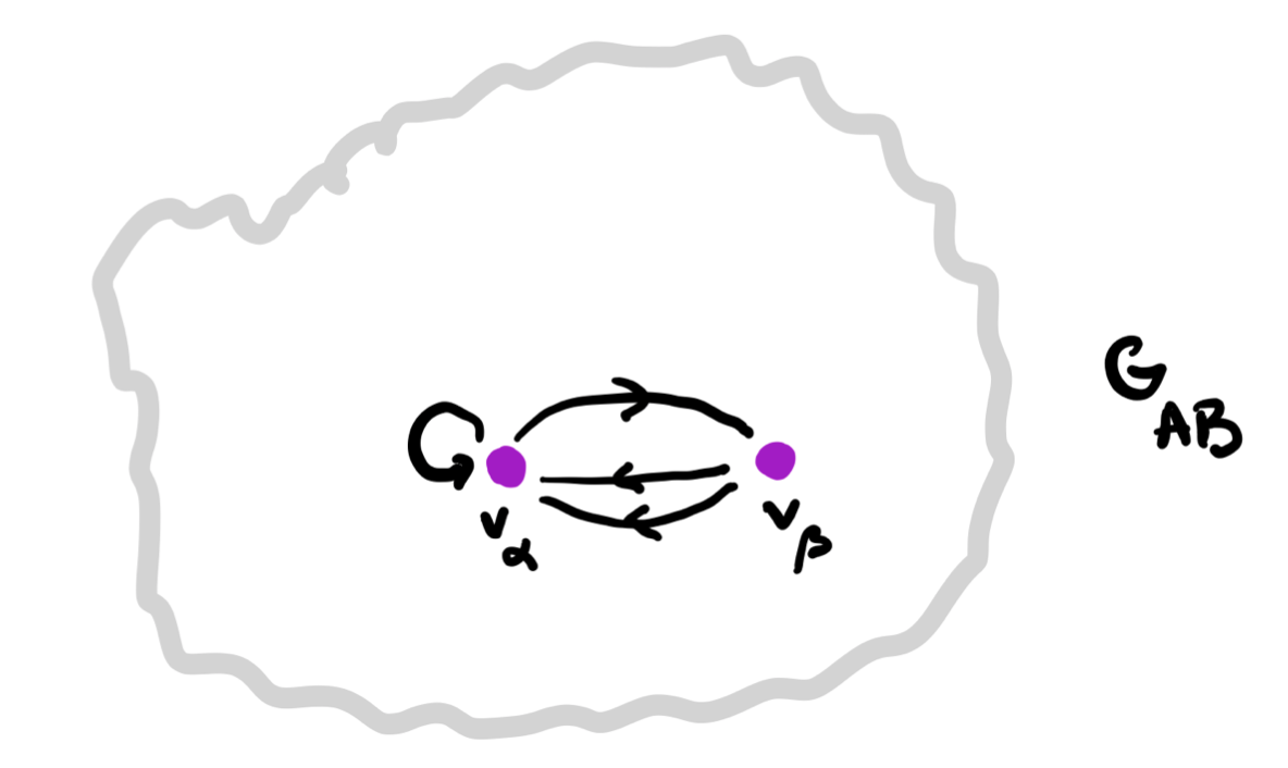
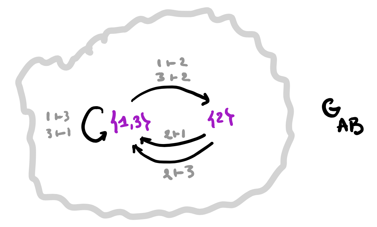
Here’s the directed graph $G_{AB}$:
- vertices $v_{\chi}$ correspond to the different $C$-labelings of $T$, one $C$-labeled rooted tree $T_{\chi}$ for every map $\chi : vtx(T) \rightarrow C$,
- arrows $v_{\chi} \rightarrow v_{\omega}$ if and only if $T_{\omega}$ is the rooted $C$-labelled tree isomorphic to the subtree of $T_{\chi}$ rooted at one step from the root.
A learner $\mathbf{A \rightarrow B}$ gives a set-valued representation of $\mathbf{G_{AB}}$.
We saw that a learner $A \rightarrow B$ is the same thing as a morphism in $\mathbf{Poly}$
\[
\varphi = (\varphi_1,\varphi[-])~:~P y^P \rightarrow C y^{A \times B} \]
with $P$ the parameter set of maps.
Here’s what we have to do:
1. Draw the directed graph on vertices $p \in P$ giving the dynamics of the morphism $\varphi$. This graph describes how the learner can cycle through the parameter-set.
2. Use the map $\varphi_1$ to label the vertices with elements from $C$.
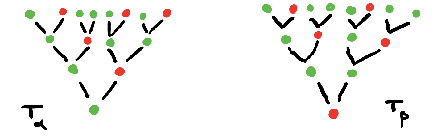
3. For each vertex draw the rooted $C$-labeled tree of potential time-evolutions starting in that vertex.
In this example the time-evolutions of the two green vertices are the same, but in general they can be different.
4. Find the vertices in $G_{AB}$ determined by these $C$-labeled trees and note that they span a full subgraph of $G_{AB}$.
5. The vertex-set $P_v$ consists of all elements from $p$ whose ($C$-labeled) vertex has evolution-tree $T_v$. If $v \rightarrow w$ is a directed edge in $G_{AB}$ corresponding to an element $(a,b) \in A \times B$, then the map on the vertex-sets corresponding to this edge is
\[
f_{v,(a,b)}~:~P_v \rightarrow P_w \qquad p \mapsto \varphi[\varphi_1(p)](a,b) \]
A set-valued representation of $\mathbf{G_{AB}}$ gives a learner $\mathbf{A \rightarrow B}$.
1. Take a set-valued representation of $G_{AB}$, that is, the finite or infinite collection of vertices $V$ in $G_{AB}$ where the vertex-set $P_v$ is non-empty. Note that these vertices span a full subgraph of $G_{AB}$.
And, for each directed arrow $v \rightarrow w$ in this subgraph, labeled by an element $(a,b) \in A \times B$ we have a map
\[
f_{v,(a,b)}~:~P_v \rightarrow P_w \]
2. The parameter set of our learner will be $P = \sqcup_v P_v$, the disjoint union of the non-empty vertex-sets.
3. The space-map $\varphi_1 : P \rightarrow C$ will send an element in $P_v$ to the $C$-label of the root of the tree $T_v$. This gives us already the interpretation and request maps
\[
I : P \times A \rightarrow B \quad \text{and} \quad R : P \times A \times B \rightarrow A \]
4. The update map $U : P \times A \times B \rightarrow P$ follows from the sheaf-map we can define stalk-wise
\[
\varphi[\varphi_1(p)](a,b) = f_{v,(a,b)}(p) \]
if $p \in P_v$.
That’s all folks!
$\mathbf{Learn(A,B)}$ is equivalent to the (covariant) functors $\mathbf{G_{AB} \rightarrow Sets}$.
Changing the directions of all arrows in $G_{AB}$ any covariant functor $\mathbf{G_{AB} \rightarrow Sets}$ becomes a contravariant functor $\mathbf{G_{AB}^o \rightarrow Sets}$, making $\mathbf{Learn(A,B)}$ an honest to Groth topos!
Every topos comes with its own logic, so we have a ‘learners’ logic’. (to be continued)
One Comment