Skip to content →

Tag: Conway

a SNORTgo endgame

SNORT, invented by Simon NORTon is a map-coloring game, similar to COL. Only, this time, neighbours may not be coloured differently.

SNORTgo, similar to COLgo, is SNORT played with go-stones on a go-board. That is, adjacent stones must have the same colour.

SNORT is a ‘hot’ game, meaning that each player is eager to move as most moves will improve your position. In COL players are reluctant to move, because a move limits your next moves.

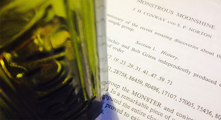
For this reason, SNORT positions are much harder to evaluate, and one needs the full force of Conways’s ONAG.

Here’s a SNORTgo endgame. Who has a winning strategy?, and what is the first move in that strategy?

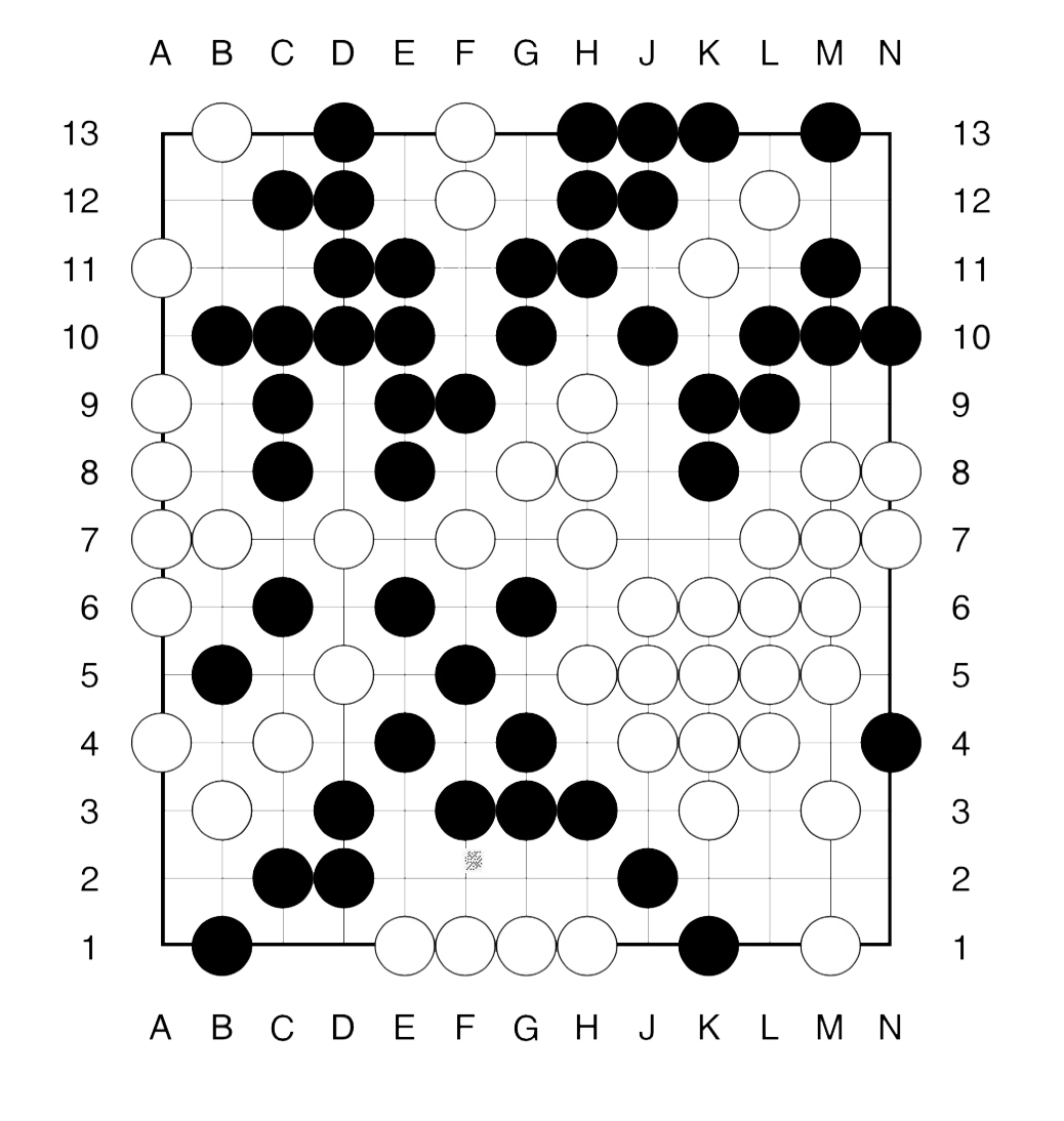
The method to approach such an endgame is similar to that in COLgo. First we remove all dead spots from the board.

What remains, are a 4 spots available only to Right (white) and 5 spots available only to Left (bLack). Further, there a 3 ‘live’ regions: the upper righthand corner and the two lower corners.

The value of these corners must be computed inductively.

Here’s the answer:

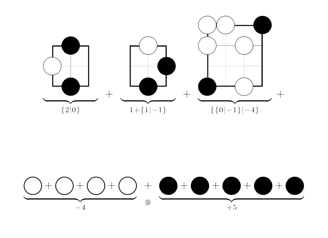
For example, Right’s best option in the left-most game (corresponding to the upper righthand corner of the endgame) is to put his stone on N12, resulting in a game in which neither player can move (the zero game).

On the other hand, Left can put a stone at either N11, N12 or N13 leaving a game in which she has two more moves, whereas Right han none (the $2$ game).

The other positions are computed similarly.

To get the value of the endgame we have to sum up all these values.

This can either be done using the addition rule given in ONAG, or by using programs in combinatorial game theory.

There’s Combinatorial Game Suite, developed by Aaron Siegel. But, for some reason I can no longer use it on macOS High Sierra.

Fortunately, the older program David Wolfe’s toolkit is still available, and runs on my MacBook.

The sum game evaluates to $\{ \{3|2 \}|-1 \}$, which is a ‘fuzzy’ game, that is, its value is confused with $0$.

This means that the first player to move has a winning strategy in the endgame.

Can you spot the (unique) winning move for Right (white) and one (of two) winning move for Left (bLack)?

Spoiler alert : solution in the comments.

One Comment

a non-commutative Jack Daniels problem

At a seminar at the College de France in 1975, Tits wrote down the order of the monster group

\[
\# \mathbb{M} = 2^{46}.3^{20}.5^9.7^6.11^2.13^3.17·19·23·29·31·41·47·59·71 \]

Andrew Ogg, who attended the talk, noticed that the prime divisors are precisely the primes $p$ for which the characteristic $p$ super-singular $j$-invariants are all defined over $\mathbb{F}_p$.

Here’s Ogg’s paper on this: Automorphismes de courbes modulaires, Séminaire Delange-Pisot-Poitou. Théorie des nombres, tome 16, no 1 (1974-1975).

Ogg offered a bottle of Jack Daniels for an explanation of this coincidence.

Even Richard Borcherds didn’t claim the bottle of Jack Daniels, though his proof of the monstrous moonshine conjecture is believed to be the best explanation, at present.

A few years ago, John Duncan and Ken Ono posted a paper “The Jack Daniels Problem”, in which they prove that monstrous moonshine implies that if $p$ is not one of Ogg’s primes it cannot be a divisor of $\# \mathbb{M}$. However, the other implication remains mysterious.

Duncan and Ono say:

“This discussion does not prove that every $p ∈ \text{Ogg}$ divides $\# \mathbb{M}$. It merely explains how the first principles of moonshine suggest this implication. Monstrous moonshine is the proof. Does this then provide a completely satisfactory solution to Ogg’s problem? Maybe or maybe not. Perhaps someone will one day furnish a map from the characteristic $p$ supersingular $j$-invariants to elements of order $p$ where the group structure of $\mathbb{M}$ is apparent.”

I don’t know whether they claimed the bottle, anyway.

But then, what is the non-commutative Jack Daniels Problem?

A footnote on the first page of Conway and Norton’s ‘Monstrous Moonshine’ paper says:

“Very recently, A. Pizer has shown these primes are the only ones that satisfy a certain conjecture of Hecke from 1936 relating modular forms of weight $2$ to quaternion algebra theta-series.”

Pizer’s paper is “A note on a conjecture of Hecke”.

Maybe there’s a connection between monstrous moonshine and the arithmetic of integral quaternion algebras. Some hints:

The commutation relations in the Big Picture are reminiscent of the meta-commutation relations for Hurwitz quaternions, originally due to Conway in his booklet on Quaternions and Octonions.

The fact that the $p$-tree in the Big Picture has valency $p+1$ comes from the fact that the Brauer-Severi of $M_2(\mathbb{F}_p)$ is $\mathbb{P}^1_{\mathbb{F}_p}$. In fact, the Big Picture should be related to the Brauer-Severi scheme of $M_2(\mathbb{Z})$.

Then, there’s Jorge Plazas claiming that Connes-Marcolli’s $GL_2$-system might be related to moonshine.

One of the first things I’ll do when I return is to run to the library and get our copy of Shimura’s ‘Introduction to the arithmetic theory of automorphic functions’.

Btw. the bottle in the title image is not a Jack Daniels but the remains of a bottle of Ricard, because I’m still in the French mountains.

Comments closed

the monstrous moonshine picture – 2

Time to wrap up my calculations on the moonshine picture, which is the subgraph of Conway’s Big Picture needed to describe all 171 moonshine groups.

No doubt I’ve made mistakes. All corrections are welcome. The starting point is the list of 171 moonshine groups which are in the original Monstrous Moonshine paper.

The backbone is given by the $97$ number lattices, which are closed under taking divisors and were found by looking at all divisors of the numbers $N=n \times h$ for the 171 moonshine groups of the form $N+e,f,\dots$ or $(n|h)+e,f,\dots$.

The Hasse-diagram of this poset (under division) is here (click on the image to get a larger version)

There are seven types of coloured numbers, each corresponding to number-lattices which have the same local structure in the moonshine picture, as in the previous post.

The white numbered lattices have no further edges in the picture.

The yellow number lattices (2,10,14,18,22,26,32,34,40,68,80,88,90,112,126,144,180,208 = 2M) have local structure

\[
\xymatrix{& \color{yellow}{2M} \ar@{-}[r] & M \frac{1}{2}} \]

The green number lattices (3,15,21,39,57,93,96,120 = 3M) have local structure

\[
\xymatrix{M \frac{1}{3} \ar@[red]@{-}[r] & \color{green}{3M} \ar@[red]@{-}[r] & M \frac{2}{3}} \]

The blue number lattices (4,16,20,28,36,44,52,56,72,104 = 4M) have as local structure

\[
\xymatrix{M \frac{1}{2} \ar@{-}[d] & & M \frac{1}{4} \ar@{-}[d] \\
2M \ar@{-}[r] & \color{blue}{4M} \ar@{-}[r] & 2M \frac{1}{2} \ar@{-}[d] \\
& & M \frac{3}{4}} \]

where the leftmost part is redundant as they are already included in the yellow-bit.

The purple number lattices (6,30,42,48,60 = 6M) have local structure

\[
\xymatrix{M \frac{1}{3} \ar@[red]@{-}[d] & 2M \frac{1}{3} & M \frac{1}{6} \ar@[red]@{-}[d] & \\
3M \ar@{-}[r] \ar@[red]@{-}[d] & \color{purple}{6M} \ar@{-}[r] \ar@[red]@{-}[u] \ar@[red]@{-}[d] & 3M \frac{1}{2} \ar@[red]@{-}[r] \ar@[red]@{-}[d] & M \frac{5}{6} \\
M \frac{2}{3} & 2M \frac{2}{3} & M \frac{1}{2} & } \]

where again the lefmost part is redundant, and I forgot to add the central part in the previous post… (updated now).

The unique brown number lattice 8 has local structure

\[
\xymatrix{& & 1 \frac{1}{4} \ar@{-}[d] & & 1 \frac{1}{8} \ar@{-}[d] & \\
& 1 \frac{1}{2} \ar@{-}[d] & 2 \frac{1}{2} \ar@{-}[r] \ar@{-}[d] & 1 \frac{3}{4} & 2 \frac{1}{4} \ar@{-}[r] & 1 \frac{5}{8} \\
1 \ar@{-}[r] & 2 \ar@{-}[r] & 4 \ar@{-}[r] & \color{brown}{8} \ar@{-}[r] & 4 \frac{1}{2} \ar@{-}[d] \ar@{-}[u] & \\
& & & 1 \frac{7}{8} \ar@{-}[r] & 2 \frac{3}{4} \ar@{-}[r] & 1 \frac{3}{8}} \]

The local structure in the two central red number lattices (not surprisingly 12 and 24) looks like the image in the previous post, but I have to add some ‘forgotten’ lattices.

That’ll have to wait…

Comments closed