These three ideas (re)surfaced over the last two decades, claiming to have potential applications to major open problems:
(2000) $\mathbb{F}_1$-geometry tries to view $\mathbf{Spec}(\mathbb{Z})$ as a curve over the field with one element, and mimic Weil’s proof of RH for curves over finite fields to prove the Riemann hypothesis.
(2014) topos theory : Connes and Consani redirected their RH-attack using arithmetic sites, while Lafforgue advocated the use of Caramello’s bridges for unification, in particular the Langlands programme.
It is difficult to voice an opinion about the (presumed) current state of such projects without being accused of being either a believer or a skeptic, resorting to group-think or being overly critical.
We lack the vocabulary to talk about the different phases a mathematical idea might be in.
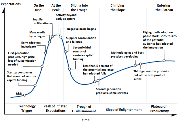
Such a vocabulary exists in (information) technology, the five phases of the Gartner hype cycle to represent the maturity, adoption, and social application of a certain technology :
Technology Trigger
Peak of Inflated Expectations
Trough of Disillusionment
Slope of Enlightenment
Plateau of Productivity
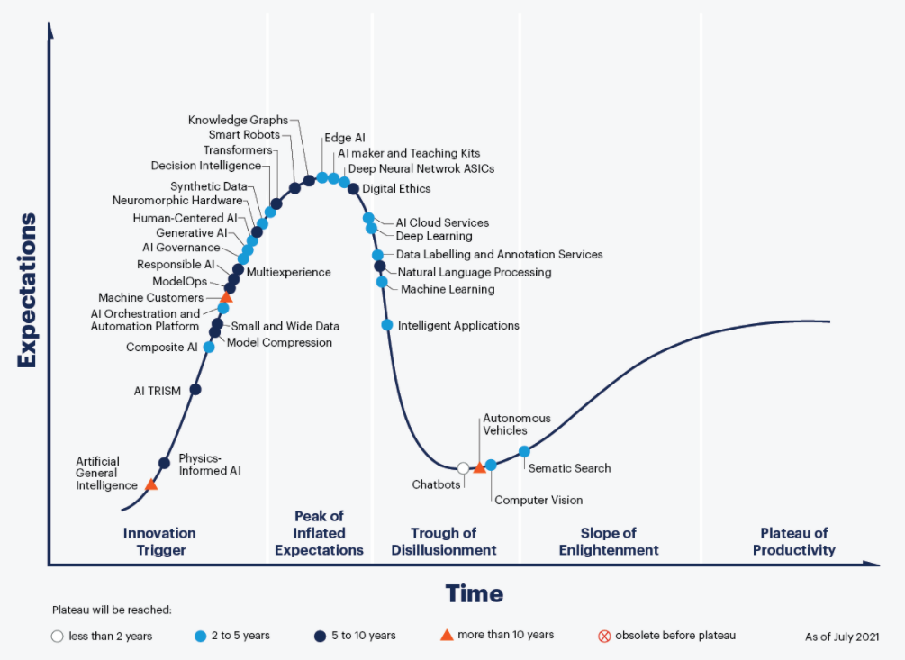
This model can then be used to gauge in which phase several emerging technologies are, and to estimate the time it will take them to reach the stable plateau of productivity. Here’s Gartner’s recent Hype Cycle for emerging Artificial Intelligence technologies.
What might these phases be in the hype cycle of a mathematical idea?
Technology Trigger: a new idea or analogy is dreamed up, marketed to be the new approach to that problem. A small group of enthusiasts embraces the idea, and tries to supply proper definitions and the very first results.
Peak of Inflated Expectations: the idea spreads via talks, blogposts, mathoverflow and twitter, and now has enough visibility to justify the first conferences devoted to it. However, all this activity does not result in major breakthroughs and doubt creeps in.
Trough of Disillusionment: the project ran out of steam. It becomes clear that existing theories will not lead to a solution of the motivating problem. Attempts by key people to keep the idea alive (by lengthy papers, regular meetings or seminars) no longer attract new people to the field.
Slope of Enlightenment: the optimistic scenario. One abandons the original aim, ditches the myriad of theories leading nowhere, regroups and focusses on the better ideas the project delivered.
A negative scenario is equally possible. Apart for a few die-hards the idea is abandoned, and on its way to the graveyard of forgotten ideas.
Plateau of Productivity: the polished surviving theory has applications in other branches and becomes a solid tool in mathematics.
It would be fun so see more knowledgable people draw such a hype cycle graph for recent trends in mathematics.
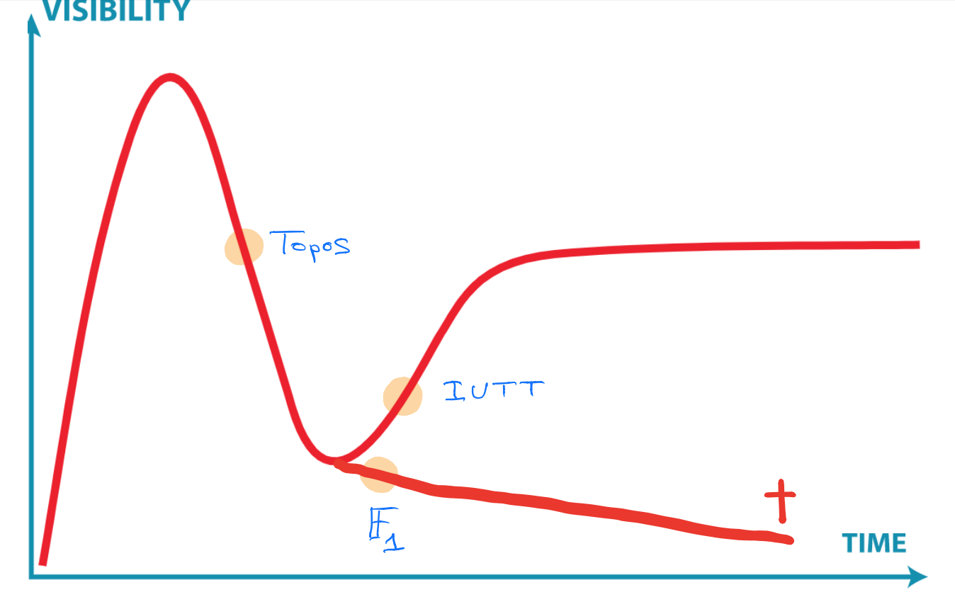
Here’s my own (feeble) attempt to gauge where the three ideas mentioned at the start are in their cycles, and here’s why:
IUTT: recent work of Kirti Joshi, for example this, and this, and that, draws from IUTT while using conventional language and not making exaggerated claims.
$\mathbb{F}_1$: the preliminary programme of their seminar shows little evidence the $\mathbb{F}_1$-community learned from the past 20 years.
Topos: Developing more general theory is not the way ahead, but concrete examples may carry surprises, even though Gabriel’s topos will remain elusive.
Clearly, you don’t agree, and that’s fine. We now have a common terminology, and you can point me to results or events I must have missed, forcing me to redraw my graph.
Here’s a nice introduction to neural networks for category theorists by Bruno Gavranovic. At 1.49m he tries to explain supervised learning with neural networks in one slide. Learners show up later in the talk.
$\mathbf{Poly}$ is the category of all polynomial functors, that is, things of the form
\[
p = \sum_{i \in p(1)} y^{p[i]}~:~\mathbf{Sets} \rightarrow \mathbf{Sets} \qquad S \mapsto \bigsqcup_{i \in p(1)} Maps(p[i],S) \]
with $p(1)$ and all $p[i]$ sets.
Last time I gave Spivak’s ‘corolla’ picture to think about such functors.
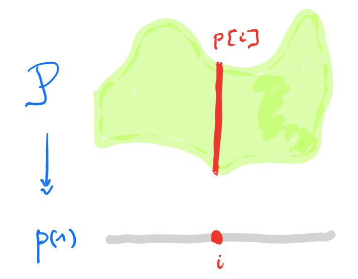
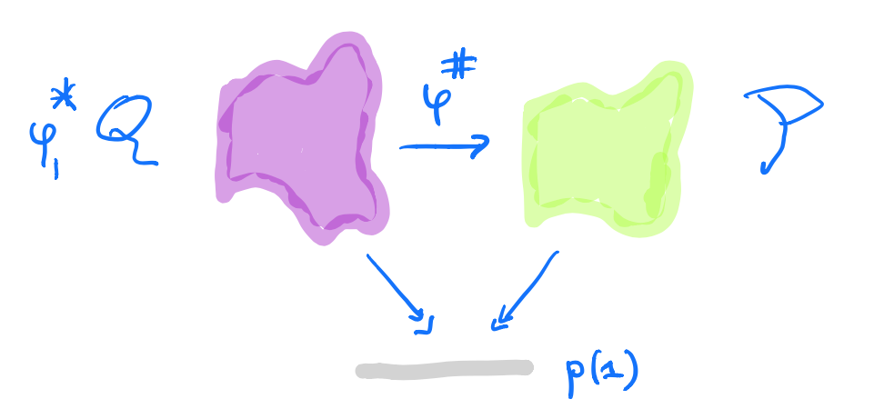
I prefer to view $p \in \mathbf{Poly}$ as an horribly discrete ‘sheaf’ $\mathcal{P}$ over the ‘space’ $p(1)$ with stalk $p[i]=\mathcal{P}_i$ at point $i \in p(1)$.
A morphism $p \rightarrow q$ in $\mathbf{Poly}$ is a map $\varphi_1 : p(1) \rightarrow q(1)$, together with for all $i \in p(1)$ a map $\varphi^{\#}_i : q[\varphi_1(i)] \rightarrow p[i]$.
In the sheaf picture, this gives a map of sheaves over the space $p(1)$ from the inverse image sheaf $\varphi_1^* \mathcal{Q}$ to $\mathcal{P}$.
But, unless you dream of sheaves in the night, by all means stick to Spivak’s corolla picture.
A learner $A \rightarrow B$ between two sets $A$ and $B$ is a complicated tuple of things $(P,I,U,R)$:
$P$ is a set, a parameter space of some maps from $A$ to $B$.
$I$ is the interpretation map $I : P \times A \rightarrow B$ describing the maps in $P$.
$U$ is the update map $U : P \times A \times B \rightarrow P$, the learning procedure. The idea is that $U(p,a,b)$ is a map which sends $a$ closer to $b$ than the map $p$ did.
$R$ is the request map $R : P \times A \times B \rightarrow A$.
Here’s a nice application of $\mathbf{Poly}$’s set-up:
Morphisms $\mathbf{P y^P \rightarrow Maps(A,B) \times Maps(A \times B,A) y^{A \times B}}$ in $\mathbf{Poly}$ coincide with learners $\mathbf{A \rightarrow B}$ with parameter space $\mathbf{P}$.
This follows from unpacking the definition of morphism in $\mathbf{Poly}$ and the process CT-ers prefer to call Currying.
The space-map $\varphi_1 : P \rightarrow Maps(A,B) \times Maps(A \times B,A)$ gives us the interpretation and request-map, whereas the sheaf-map $\varphi^{\#}$ gives us the more mysterious update-map $P \times A \times B \rightarrow P$.
$\mathbf{Learn(A,B)}$ is the category with objects all the learners $A \rightarrow B$ (for all paramater-sets $P$), and with morphisms defined naturally, that is, maps between the parameter-sets, compatible with the structural maps.
$\mathbf{Learn(A,B)}$ is a topos. In fact, it is the topos of all set-valued representations of a (huge) directed graph $\mathbf{G_{AB}}$.
This will take some time.
Let’s bring some dynamics in. Take any polynmial functor $p \in \mathbf{Poly}$ and fix a morphism in $\mathbf{Poly}$
\[
\varphi = (\varphi_1,\varphi[-])~:~p(1) y^{p(1)} \rightarrow p \]
with space-map $\varphi_1$ the identity map.
We form a directed graph:
the vertices are the elements of $p(1)$,
vertex $i \in p(1)$ is the source vertex of exactly one arrow for every $a \in p[i]$,
the target vertex of that arrow is the vertex $\phi[i](a) \in p(1)$.
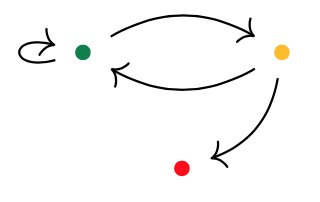
Here’s one possibility from Spivak’s paper for $p = 2y^2 + 1$, with the coefficient $2$-set $\{ \text{green dot, yellow dot} \}$, and with $1$ the singleton $\{ \text{red dot} \}$.
Start at one vertex and move after a minute along a directed edge to the next (possibly the same) vertex. The potential evolutions in time will then form a tree, with each node given a label in $p(1)$.
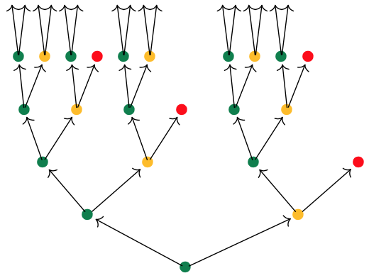
If we start at the green dot, we get this tree of potential time-evolutions
There are exactly $\# p[i]$ branches leaving a node labeled $i \in p(1)$, and all subtrees emanating from equal labelled nodes are isomorphic.
If we had started at the yellow dot we had obtained a labelled tree isomorphic to the subtree emanating here from any yellow dot.
We can do the same things for any morphism in $\mathbf{Poly}$ of the form
\[
\varphi = (\varphi_1,\varphi[-])~:~Sy^S \rightarrow p \]
Now, we have a directed graph with vertices the elements $s \in S$, with as many edges leaving vertex $s$ as there are elements $a \in p[\varphi_1(s)]$, and with the target vertex of the edge labeled $a$ starting in $s$ the vertex $\varphi[\varphi_1(s)](A)$.
Once we have this directed graph on $\# S$ vertices we can label vertex $s$ with the label $\varphi_1(s)$ from $p(1)$.
In this way, the time evolutions starting at a vertex $s \in S$ will give us a $p(1)$-labelled rooted tree.
But now, it is possibly that two distinct vertices can have the same $p(1)$-labeled tree of evolutions. But also, trees corresponding to equal labeled vertices can be different.
Right, I guess we’re ready to define the graph $G_{AB}$ and prove that $\mathbf{Learn(A,B)}$ is a topos.
In the case of learners, we have the target polynomial functor $p=C y^{A \times B}$ with $C = Maps(A,B) \times Maps(A \times B,A)$, that is
\[
p(1) = C \quad \text{and all} \quad p[i]=A \times B \]
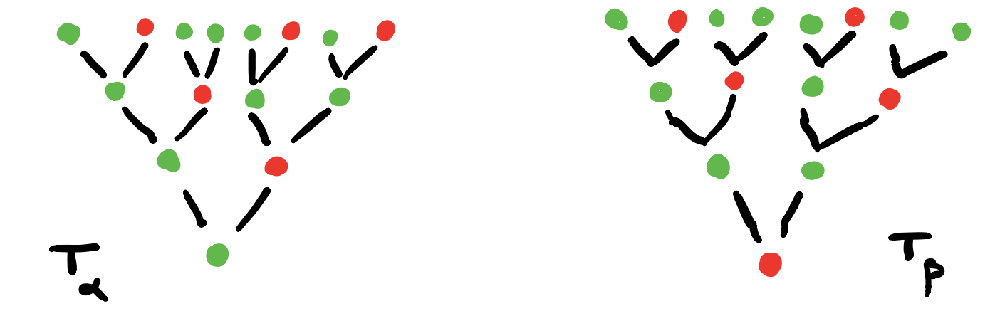
Start with the free rooted tree $T$ having exactly $\# A \times B$ branches growing from each node.
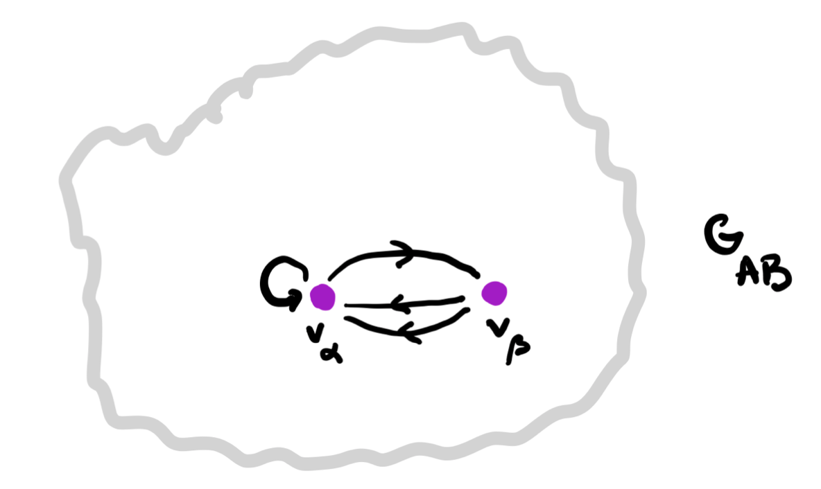
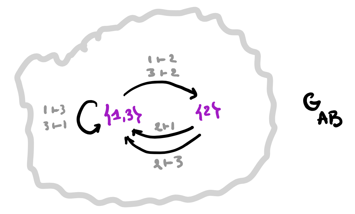
Here’s the directed graph $G_{AB}$:
vertices $v_{\chi}$ correspond to the different $C$-labelings of $T$, one $C$-labeled rooted tree $T_{\chi}$ for every map $\chi : vtx(T) \rightarrow C$,
arrows $v_{\chi} \rightarrow v_{\omega}$ if and only if $T_{\omega}$ is the rooted $C$-labelled tree isomorphic to the subtree of $T_{\chi}$ rooted at one step from the root.
A learner $\mathbf{A \rightarrow B}$ gives a set-valued representation of $\mathbf{G_{AB}}$.
We saw that a learner $A \rightarrow B$ is the same thing as a morphism in $\mathbf{Poly}$
\[
\varphi = (\varphi_1,\varphi[-])~:~P y^P \rightarrow C y^{A \times B} \]
with $P$ the parameter set of maps.
Here’s what we have to do:
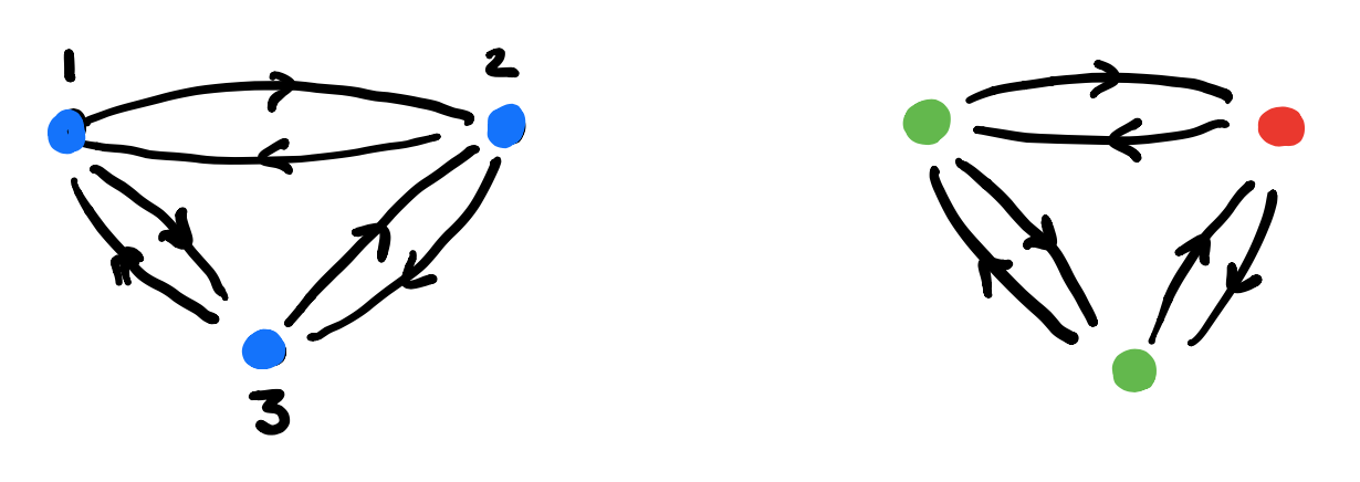
1. Draw the directed graph on vertices $p \in P$ giving the dynamics of the morphism $\varphi$. This graph describes how the learner can cycle through the parameter-set.
2. Use the map $\varphi_1$ to label the vertices with elements from $C$.
3. For each vertex draw the rooted $C$-labeled tree of potential time-evolutions starting in that vertex.
In this example the time-evolutions of the two green vertices are the same, but in general they can be different.
4. Find the vertices in $G_{AB}$ determined by these $C$-labeled trees and note that they span a full subgraph of $G_{AB}$.
5. The vertex-set $P_v$ consists of all elements from $p$ whose ($C$-labeled) vertex has evolution-tree $T_v$. If $v \rightarrow w$ is a directed edge in $G_{AB}$ corresponding to an element $(a,b) \in A \times B$, then the map on the vertex-sets corresponding to this edge is
\[
f_{v,(a,b)}~:~P_v \rightarrow P_w \qquad p \mapsto \varphi[\varphi_1(p)](a,b) \]
A set-valued representation of $\mathbf{G_{AB}}$ gives a learner $\mathbf{A \rightarrow B}$.
1. Take a set-valued representation of $G_{AB}$, that is, the finite or infinite collection of vertices $V$ in $G_{AB}$ where the vertex-set $P_v$ is non-empty. Note that these vertices span a full subgraph of $G_{AB}$.
And, for each directed arrow $v \rightarrow w$ in this subgraph, labeled by an element $(a,b) \in A \times B$ we have a map
\[
f_{v,(a,b)}~:~P_v \rightarrow P_w \]
2. The parameter set of our learner will be $P = \sqcup_v P_v$, the disjoint union of the non-empty vertex-sets.
3. The space-map $\varphi_1 : P \rightarrow C$ will send an element in $P_v$ to the $C$-label of the root of the tree $T_v$. This gives us already the interpretation and request maps
\[
I : P \times A \rightarrow B \quad \text{and} \quad R : P \times A \times B \rightarrow A \]
4. The update map $U : P \times A \times B \rightarrow P$ follows from the sheaf-map we can define stalk-wise
\[
\varphi[\varphi_1(p)](a,b) = f_{v,(a,b)}(p) \]
if $p \in P_v$.
That’s all folks!
$\mathbf{Learn(A,B)}$ is equivalent to the (covariant) functors $\mathbf{G_{AB} \rightarrow Sets}$.
Changing the directions of all arrows in $G_{AB}$ any covariant functor $\mathbf{G_{AB} \rightarrow Sets}$ becomes a contravariant functor $\mathbf{G_{AB}^o \rightarrow Sets}$, making $\mathbf{Learn(A,B)}$ an honest to Groth topos!
Every topos comes with its own logic, so we have a ‘learners’ logic’. (to be continued)
Scholze and Clausen ran a masterclass in Copenhagen on condensed mathematics, which you can binge watch on YouTube starting here
Scholze also gave two courses on the material in Bonn of which the notes are available here and here.
Condensed mathematics claims that topological spaces are the wrong definition, and that one should replace them with the slightly different notion of condensed sets.
So, let’s find out what a condensed set is.
Definition: Condensed sets are sheaves (of sets) on the pro-étale site of a point.
(there’s no danger we’ll have to rewrite our undergraduate topology courses just yet…)
In his blogpost, Scholze motivates this paradigm shift by observing that the category of topological Abelian groups is not Abelian (if you put a finer topology on the same group then the identity map is not an isomorphism but doesn’t have a kernel nor cokernel) whereas the category of condensed Abelian groups is.
It was another Clausen-Scholze result in the blogpost that caught my eye.
Exhibiting the open question = to understand the object $A$
Identifying the semiotic context = to describe the category $\mathbf{C}$ of which $A$ is an object
Finding the question’s critical sign = $A$ (?!)
Identifying the concept’s walls = the uncontrolled behaviour of the Yoneda functor
\[
@A~:~\mathbf{C} \rightarrow \mathbf{Sets} \qquad C \mapsto Hom_{\mathbf{C}}(C,A) \]
Opening the walls = finding an objectively creative subcategory $\mathbf{A}$ of $\mathbf{C}$
Displaying extended wall perspectives = calculate the colimit $C$ of a creative diagram
Evaluating the extended walls = try to understand $A$ via the isomorphism $C \simeq A$.
The creative moment comes in here: could we not find a subcategory
$\mathbf{A}$ of $\mathbf{C}$ such that the functor
\[
Yon|_{\mathbf{A}}~:~\mathbf{C} \rightarrow \mathbf{PSh}(\mathbf{A}) \qquad A \mapsto @A|_{\mathbf{A}} \]
is still fully faithful? We call such a subcategory creative, and it is a major task in category theory to find creative categories which are as small as possible.
All the ingredients are here, but I had to read Peter Scholze’s blogpost before the penny dropped.
Let’s try to view condensed sets as the result of a creative process.
Exhibiting the open question: you are a topologist and want to understand a particular compact Hausdorff space $X$.
Identifying the semiotic context: you are familiar with working in the category $\mathbf{Tops}$ of all topological spaces with continuous maps as morphisms.
Finding the question’s critical sign: you want to know what differentiates your space $X$ from all other topological spaces.
Identifying the concept’s walls: you can probe your space $X$ with continuous maps from other topological spaces. That is, you can consider the contravariant functor (or presheaf on $\mathbf{Tops}$)
\[
@X~:~\mathbf{Tops} \rightarrow \mathbf{Sets} \qquad Y \mapsto Cont(Y,X) \]
and Yoneda tells you that this functor, up to equivalence, determines the space $X$ upto homeomorphism.
Opening the walls: Tychonoff tells you that among all compact Hausdorff spaces there’s a class of pretty weird examples: inverse limits of finite sets (or a bit pompous: the pro-etale site of a point). These limits form a subcategory $\mathbf{ProF}$ of $\mathbf{Tops}$.
Displaying extended wall perspectives: for every inverse limit $F \in \mathbf{ProF}$ (for ‘pro-finite sets’) you can look at the set $\mathbf{X}(F)=Cont(F,X)$ of all continuous maps from $F$ to $X$ (that is, all probes of $X$ by $F$) and this functor
\[
\mathbf{X}=@X|_{\mathbf{ProF}}~:~\mathbf{ProF} \rightarrow \mathbf{Sets} \qquad F \mapsto \mathbf{X}(F) \]
is a sheaf on the pre-etale site of a point, that is, $\mathbf{X}$ is the condensed set associated to $X$.
Evaluating the extended walls: Clausen and Scholze observe that the assignment $X \mapsto \mathbf{X}$ embeds compact Hausdorff spaces fully faithful into condensed sets, so we can recover $X$ up to homeomorphism as a colimit from the condenset set $\mathbf{X}$. Or, in Mazzola’s terminology: $\mathbf{ProF}$ is a creative subcategory of $\mathbf{(cH)Tops}$ (all compact Hausdorff spaces).
It would be nice if someone would come up with a new notion for me to understand Mazzola’s other opus “The topos of music” (now reprinted as a four volume series).