Tag: Riemann

Klein’s dessins d’enfant and the buckyball

Published June 30, 2008 by lieven

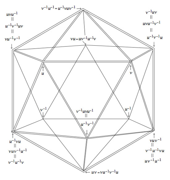
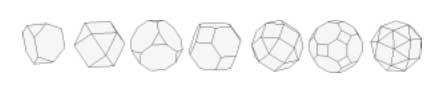
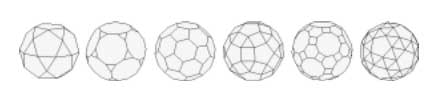
We saw that the icosahedron can be constructed from the alternating group $A_{5}$ by considering the elements of a conjugacy class of order 5 elements as the vertices and edges between two vertices if their product is still in the conjugacy class.

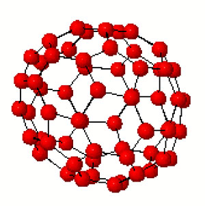
This description is so nice that one would like to have a similar construction for the buckyball. But, the buckyball has 60 vertices, so they surely cannot correspond to the elements of a conjugacy class of $A_{5}$ . But, perhaps there is a larger group, somewhat naturally containing $A_{5}$ , having a conjugacy class of 60 elements?

This is precisely the statement contained in Galois’ last letter. He showed that 11 is the largest prime p such that the group $L_{2} (p) = P S L_{2} (F_{p})$ has a (transitive) permutation presentation on p elements. For, p=11 the group $L_{2} (11)$ is of order 660, so it permuting 11 elements means that this set must be of the form $X = L_{2} (11) / A$ with $A \subset L_{2} (11)$ a subgroup of 60 elements… and it turns out that $A ≃ A_{5}$ …

Actually there are TWO conjugacy classes of subgroups isomorphic to $A_{5}$ in $L_{2} (11)$ and we have already seen one description of these using the biplane geometry (one class is the stabilizer subgroup of a ‘line’, the other the stabilizer subgroup of a point).

Here, we will give yet another description of these two classes of $A_{5}$ in $L_{2} (11)$ , showing among other things that the theory of dessins d’enfant predates Grothendieck by 100 years.

In the very same paper containing the first depiction of the Dedekind tessellation, Klein found that there should be a degree 11 cover $P_{C}^{1} \to P_{C}^{1}$ with monodromy group $L_{2} (11)$ , ramified only in the three points $0, 1, \infty$ such that there is just one point lying over $\infty$ , seven over 1 of which four points where two sheets come together and finally 5 points lying over 0 of which three where three sheets come together. In 1879 he wanted to determine this cover explicitly in the paper “Ueber die Transformationen elfter Ordnung der elliptischen Funktionen” (Math. Annalen) by describing all Riemann surfaces with this ramification data and pick out those with the correct monodromy group.

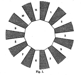
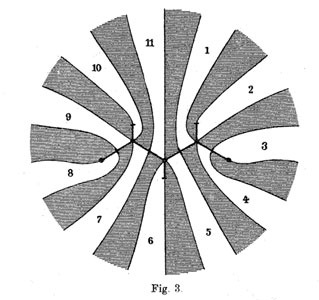
He manages to do so by associating to all these covers their ‘dessins d’enfants’ (which he calls Linienzuges), that is the pre-image of the interval [0,1] in which he marks the preimages of 0 by a bullet and those of 1 by a +, such as in the innermost darker graph on the right above. He even has these two wonderful pictures explaining how the dessin determines how the 11 sheets fit together. (More examples of dessins and the correspondences of sheets were drawn in the 1878 paper.)

The ramification data translates to the following statements about the Linienzuge : (a) it must be a tree ( $\infty$ has one preimage), (b) there are exactly 11 (half)edges (the degree of the cover),
(c) there are 7 +-vertices and 5 o-vertices (preimages of 0 and 1) and (d) there are 3 trivalent o-vertices and 4 bivalent +-vertices (the sheet-information).

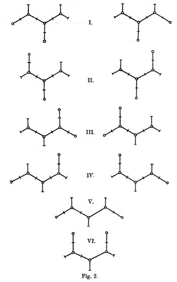
Klein finds that there are exactly 10 such dessins and lists them in his Fig. 2 (left). Then, he claims that one the two dessins of type I give the correct monodromy group. Recall that the monodromy group is found by giving each of the half-edges a number from 1 to 11 and looking at the permutation $τ$ of order two pairing the half-edges adjacent to a +-vertex and the order three permutation $σ$ listing the half-edges by cycling counter-clockwise around a o-vertex. The monodromy group is the group generated by these two elements.

Fpr example, if we label the type V-dessin by the numbers of the white regions bordering the half-edges (as in the picture Fig. 3 on the right above) we get
$σ = (7, 10, 9) (5, 11, 6) (1, 4, 2)$ and $τ = (8, 9) (7, 11) (1, 5) (3, 4)$ .

Nowadays, it is a matter of a few seconds to determine the monodromy group using GAP and we verify that this group is $A_{11}$ .

Of course, Klein didn’t have GAP at his disposal, so he had to rule out all these cases by hand.

gap> g:=Group((7,10,9)(5,11,6)(1,4,2),(8,9)(7,11)(1,5)(3,4));
Group([ (1,4,2)(5,11,6)(7,10,9), (1,5)(3,4)(7,11)(8,9) ])
gap> Size(g);
19958400
gap> IsSimpleGroup(g);
true

Klein used the fact that $L_{2} (11)$ only has elements of orders 1,2,3,5,6 and 11. So, in each of the remaining cases he had to find an element of a different order. For example, in type V he verified that the element $τ . (σ . τ)^{3}$ is equal to the permutation (1,8)(2,10,11,9,6,4,5)(3,7) and consequently is of order 14.

Perhaps Klein knew this but GAP tells us that the monodromy group of all the remaining 8 cases is isomorphic to the alternating group $A_{11}$ and in the two type I cases is indeed $L_{2} (11)$ . Anyway, the two dessins of type I correspond to the two conjugacy classes of subgroups $A_{5}$ in the group $L_{2} (11)$ .

But, back to the buckyball! The upshot of all this is that we have the group $L_{2} (11)$ containing two classes of subgroups isomorphic to $A_{5}$ and the larger group $L_{2} (11)$ does indeed have two conjugacy classes of order 11 elements containing exactly 60 elements (compare this to the two conjugacy classes of order 5 elements in $A_{5}$ in the icosahedral construction). Can we construct the buckyball out of such a conjugacy class?

To start, we can identify the 12 pentagons of the buckyball from a conjugacy class C of order 11 elements. If $x \in C$ , then so do $x^{3}, x^{4}, x^{5}$ and $x^{9}$ , whereas the powers $x^{2}, x^{6}, x^{7}, x^{8}, x^{10}$ belong to the other conjugacy class. Hence, we can divide our 60 elements in 12 subsets of 5 elements and taking an element x in each of these, the vertices of a pentagon correspond (in order) to $(x, x^{3}, x^{9}, x^{5}, x^{4})$ .

Group-theoretically this follows from the fact that the factorgroup of the normalizer of x modulo the centralizer of x is cyclic of order 5 and this group acts naturally on the conjugacy class of x with orbits of size 5.

Finding out how these pentagons fit together using hexagons is a lot subtler… and in The graph of the truncated icosahedron and the last letter of Galois Bertram Kostant shows how to do this.

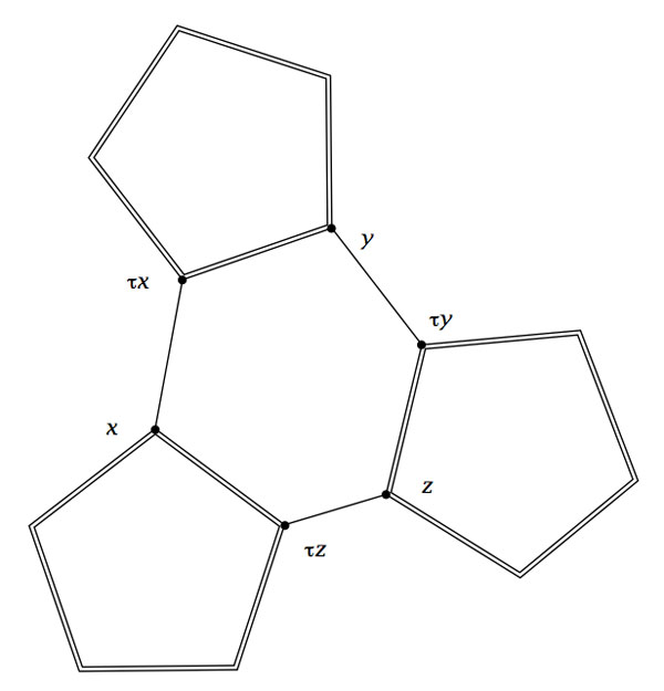
Fix a subgroup isomorphic to $A_{5}$ and let D be the set of all its order 2 elements (recall that they form a full conjugacy class in this $A_{5}$ and that there are precisely 15 of them). Now, the startling observation made by Kostant is that for our order 11 element $x$ in C there is a unique element $a \in D$ such that the commutator $b = [x, a] = x^{- 1} a^{- 1} x a$ belongs again to D. The unique hexagonal side having vertex x connects it to the element $b . x$ which belongs again to C as $b . x = (a x)^{- 1} . x . (a x)$ .

Concluding, if C is a conjugacy class of order 11 elements in $L_{2} (11)$ , then its 60 elements can be viewed as corresponding to the vertices of the buckyball. Any element $x \in C$ is connected by two pentagonal sides to the elements $x^{3}$ and $x^{4}$ and one hexagonal side connecting it to $τ x = b . x$ .

the buckyball symmetries

Published June 27, 2008 by lieven

The buckyball is without doubt the hottest mahematical object at the moment (at least in Europe). Recall that the buckyball (middle) is a mixed form of two Platonic solids

the Icosahedron on the left and the Dodecahedron on the right.

For those of you who don’t know anything about football, it is that other ball-game, best described via a quote from the English player Gary Lineker

“Football is a game for 22 people that run around, play the ball, and one referee who makes a slew of mistakes, and in the end Germany always wins.”

We still have a few days left hoping for a better ending… Let’s do some bucky-maths : what is the rotation symmetry group of the buckyball?

For starters, dodeca- and icosahedron are dual solids, meaning that if you take the center of every face of a dodecahedron and connect these points by edges when the corresponding faces share an edge, you’ll end up with the icosahedron (and conversely). Therefore, both solids (as well as their mixture, the buckyball) will have the same group of rotational symmetries. Can we at least determine the number of these symmetries?

Take the dodecahedron and fix a face. It is easy to find a rotation taking this face to anyone of its five adjacent faces. In group-slang : the rotation automorphism group acts transitively on the 12 faces of the dodecohedron. Now, how many of them fix a given face? These can only be rotations with axis through the center of the face and there are exactly 5 of them preserving the pentagonal face. So, in all we have $12 \times 5 = 60$ rotations preserving any of the three solids above. By composing two of its elements, we get another rotational symmetry, so they form a group and we would like to determine what that group is.

There is one group that springs to mind $A_{5}$ , the subgroup of all even permutations on 5 elements. In general, the alternating group has half as many elements as the full permutation group $S_{n}$ , that is $\frac{1}{2} n!$ (for multiplying with the involution (1,2) gives a bijection between even and odd permutations). So, for $A_{5}$ we get 60 elements and we can list them :

the trivial permutation $()$ , being the identity.
permutations of order two with cycle-decompostion $(i_{1}, i_{2}) (i_{3}, i_{4})$ , and there are exactly 15 of them around when all numbers are between 1 and 5.
permutations of order three with cycle-form $(i_{1}, i_{2}, i_{3})$ of which there are exactly 20.
permutations of order 5 which have to form one full cycle $(i_{1}, i_{2}, i_{3}, i_{4}, i_{5})$ . There are 24 of those.

Can we at least view these sets of elements as rotations of the buckyball? Well, a dodecahedron has 12 pentagobal faces. So there are 4 nontrivial rotations of order 5 for every 2 opposite faces and hence the dodecaheder (and therefore also the buckyball) has indeed 6×4=24 order 5 rotational symmetries.

The icosahedron has twenty triangles as faces, so any of the 10 pairs of opposite faces is responsible for two non-trivial rotations of order three, giving us 10×2=20 order 3 rotational symmetries of the buckyball.

The order two elements are slightly harder to see. The icosahedron has 30 edges and there is a plane going through each of the 15 pairs of opposite edges splitting the icosahedron in two. Hence rotating to interchange these two edges gives one rotational symmetry of order 2 for each of the 15 pairs.

And as 24+20+15+1(identity) = 60 we have found all the rotational symmetries and we see that they pair up nicely with the elements of $A_{5}$ . But do they form isomorphic groups? In other words, can the buckyball see the 5 in the group $A_{5}$ .

In a previous post I’ve shown that one way to see this 5 is as the number of inscribed cubes in the dodecahedron. But, there is another way to see the five based on the order 2 elements described before.

If you look at pairs of opposite edges of the icosahedron you will find that they really come in triples such that the planes determined by each pair are mutually orthogonal (it is best to feel this on ac actual icosahedron). Hence there are 15/3 = 5 such triples of mutually orthogonal symmetry planes of the icosahedron and of course any rotation permutes these triples. It takes a bit of more work to really check that this action is indeed the natural permutation action of $A_{5}$ on 5 elements.

Having convinced ourselves that the group of rotations of the buckyball is indeed the alternating group $A_{5}$ , we can reverse the problem : can the alternating group $A_{5}$ see the buckyball???

Well, for starters, it can ‘see’ the icosahedron in a truly amazing way. Look at the conjugacy classes of $A_{5}$ . We all know that in the full symmetric group $S_{n}$ elements belong to the same conjugacy class if and only if they have the same cycle decomposition and this is proved using the fact that the conjugation f a cycle $(i_{1}, i_{2}, \dots, i_{k})$ under a permutation $σ \in S_{n}$ is equal to the cycle $(σ (i_{1}), σ (i_{2}), \dots, σ (i_{k}))$ (and this gives us also the candidate needed to conjugate two partitions into each other).

Using this trick it is easy to see that all the 15 order 2 elements of $A_{5}$ form one conjugacy class, as do the 20 order 3 elements. However, the 24 order 5 elements split up in two conjugacy classes of 12 elements as the permutation needed to conjugate $(1, 2, 3, 4, 5)$ to $(1, 2, 3, 5, 4)$ is $(4, 5)$ but this is not an element of $A_{5}$ .

Okay, now take one of these two conjugacy classes of order 5 elements, say that of $(1, 2, 3, 4, 5)$ . It consists of 12 elements, 12 being also the number of vertices of the icosahedron. So, is there a way to identify the elements in the conjugacy class to the vertices in such a way that we can describe the edges also in terms of group-computations in $A_{5}$ ?

Surprisingly, this is indeed the case as is demonstrated in a marvelous paper by Kostant “The graph of the truncated icosahedron and the last letter of Galois”.

Two elements $a, b$ in the conjugacy class C share an edge if and only if their product $a . b \in A_{5}$ still belongs to the conjugacy class C!

So, for example $(1, 2, 3, 4, 5) . (2, 1, 4, 3, 5) = (2, 5, 4)$ so there is no edge between these elements, but on the other hand $(1, 2, 3, 4, 5) . (5, 3, 4, 1, 2) = (1, 5, 2, 4, 3)$ so there is an edge between these! It is no coincidence that $(5, 3, 4, 1, 2) = (2, 1, 4, 3, 5)^{- 1}$ as inverse elements correspond in the bijection to opposite vertices and for any pair of non-opposite vertices of an icosahedron it is true that either they are neighbors or any one of them is the neighbor of the opposite vertex of the other element.

If we take $u = (1, 2, 3, 4, 5)$ and $v = (5, 3, 4, 1, 2)$ (or any two elements of the conjugacy class such that u.v is again in the conjugacy class), then one can describe all the vertices of the icosahedron group-theoretically as follows

Isn’t that nice? Well yes, you may say, but that is just the icosahedron. Can the group $A_{5}$ also see the buckyball?

Well, let’s try a similar strategy : the buckyball has 60 vertices, exactly as many as there are elements in the group $A_{5}$ . Is there a way to connect certain elements in a group according to fixed rules? Yes, there is such a way and it is called the Cayley Graph of a group. It goes like this : take a set of generators $g_{1}, \dots, g_{k}$ of a group G, then connect two group element $a, b \in G$ with an edge if and only if $a = g_{i} . b$ or $b = g_{i} . a$ for some of the generators.

Back to the alternating group $A_{5}$ . There are several sets of generators, one of them being the elements $(1, 2, 3, 4, 5), (2, 3) (4, 5)$ . In the paper mentioned before, Kostant gives an impressive group-theoretic proof of the fact that the Cayley-graph of $A_{5}$ with respect to these two generators is indeed the buckyball!

Let us allow to be lazy for once and let SAGE do the hard work for us, and let us just watch the outcome. Here’s how that’s done

A=PermutationGroup([‘(1,2,3,4,5)’,'(2,3)(4,5)’])
B=A.cayley_graph()
B.show3d()

The outcone is a nice 3-dimensional picture of the buckyball. Below you can see a still, and, if you click on it you will get a 3-dimensional model of it (first click the ‘here’ link in the new window and then you’d better control-click and set the zoom to 200% before you rotate it)

Hence, viewing this Cayley graph from different points we have convinced ourselves that it is indeed the buckyball. In fact, most (truncated) Platonic solids appear as Cayley graphs of groups with respect to specific sets of generators. For later use here is a (partial) survey (taken from Jaap’s puzzle page)

Tetrahedron : $C_{2} \times C_{2}, [(12) (34), (13) (24), (14) (23)]$
Cube : $D_{4}, [(1234), (13)]$
Octahedron : $S_{3}, [(123), (12), (23)]$
Dodecahedron : IMPOSSIBLE
Icosahedron : $A_{4}, [(123), (234), (13) (24)]$

Truncated tetrahedron : $A_{4}, [(123), (12) (34)]$
Cuboctahedron : $A_{4}, [(123), (234)]$
Truncated cube : $S_{4}, [(123), (34)]$
Truncated octahedron : $S_{4}, [(1234), (12)]$
Rhombicubotahedron : $S_{4}, [(1234), (123)]$
Rhombitruncated cuboctahedron : IMPOSSIBLE
Snub cuboctahedron : $S_{4}, [(1234), (123), (34)]$

Icosidodecahedron : IMPOSSIBLE
Truncated dodecahedron : $A_{5}, [(124), (23) (45)]$
Truncated icosahedron : $A_{5}, [(12345), (23) (45)]$
Rhombicosidodecahedron : $A_{5}, [(12345), (124)]$
Rhombitruncated icosidodecahedron : IMPOSSIBLE
Snub Icosidodecahedron : $A_{5}, [(12345), (124), (23) (45)]$

Again, all these statements can be easily verified using SAGE via the method described before. Next time we will go further into the Kostant’s group-theoretic proof that the buckyball is the Cayley graph of $A_{5}$ with respect to (2,5)-generators as this calculation will be crucial in the description of the buckyball curve, the genus 70 Riemann surface discovered by David Singerman and
Pablo Martin which completes the trinity corresponding to the Galois trinity

Looking for F_un

Published June 3, 2008 by lieven

There are only a handful of human activities where one goes to extraordinary lengths to keep a dream alive, in spite of overwhelming evidence : religion, theoretical physics, supporting the Belgian football team and … mathematics.

In recent years several people spend a lot of energy looking for properties of an elusive object : the field with one element $F_{1}$ , or in French : “F-un”. The topic must have reached a level of maturity as there was a conference dedicated entirely to it : NONCOMMUTATIVE GEOMETRY AND GEOMETRY OVER THE FIELD WITH ONE ELEMENT.

In this series I’d like to find out what the fuss is all about, why people would like it to exist and what it has to do with noncommutative geometry. However, before we start two remarks :

The field $F_{1}$ does not exist, so don’t try to make sense of sentences such as “The ‘field with one element’ is the free algebraic monad generated by one constant (p.26), or the universal generalized ring with zero (p.33)” in the wikipedia-entry. The simplest proof is that in any (unitary) ring we have $0 \neq 1$ so any ring must contain at least two elements. A more highbrow version : the ring of integers $Z$ is the initial object in the category of unitary rings, so it cannot be an algebra over anything else.

The second remark is that several people have already written blog-posts about $F_{1}$ . Here are a few I know of : David Corfield at the n-category cafe and at his old blog, Noah Snyder at the secret blogging seminar, Kea at the Arcadian functor, AC and K. Consani at Noncommutative geometry and John Baez wrote about it in his weekly finds.

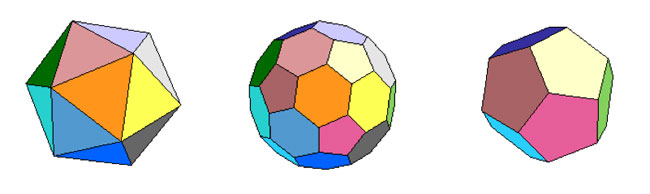
The dream we like to keep alive is that we will prove the Riemann hypothesis one fine day by lifting Weil’s proof of it in the case of curves over finite fields to rings of integers.

Even if you don’t know a word about Weil’s method, if you think about it for a couple of minutes, there are two immediate formidable problems with this strategy.

For most people this would be evidence enough to discard the approach, but, we mathematicians have found extremely clever ways for going into denial.

The first problem is that if we want to think of $spec (Z)$ (or rather its completion adding the infinite place) as a curve over some field, then $Z$ must be an algebra over this field. However, no such field can exist…

No problem! If there is no such field, let us invent one, and call it $F_{1}$ . But, it is a bit hard to do geometry over an illusory field. Christophe Soule succeeded in defining varieties over $F_{1}$ in a talk at the 1999 Arbeitstagung and in a more recent write-up of it : Les varietes sur le corps a un element.

We will come back to this in more detail later, but for now, here’s the main idea. Consider an existent field $k$ and an algebra $k \to R$ over it. Now study the properties of the functor (extension of scalars) from $k$ -schemes to $R$ -schemes. Even if there is no morphism $F_{1} \to Z$ , let us assume it exists and define $F_{1}$ -varieties by requiring that these guys should satisfy the properties found before for extension of scalars on schemes defined over a field by going to schemes over an algebra (in this case, $Z$ -schemes). Roughly speaking this defines $F_{1}$ -schemes as subsets of points of suitable $Z$ -schemes.

But, this is just one half of the story. He adds to such an $F_{1}$ -variety extra topological data ‘at infinity’, an idea he attributes to J.-B. Bost. This added feature is a $C$ -algebra $A_{X}$ , which does not necessarily have to be commutative. He only writes : “Par ignorance, nous resterons tres evasifs sur les proprietes requises sur cette $C$ -algebre.”

The algebra $A_{X}$ originates from trying to bypass the second major obstacle with the Weil-Riemann-strategy. On a smooth projective curve all points look similar as is clear for example by noting that the completions of all local rings are isomorphic to the formal power series $k [[x]]$ over the basefield, in particular there is no distinction between ‘finite’ points and those lying at ‘infinity’.

The completions of the local rings of points in $spec (Z)$ on the other hand are completely different, for example, they have residue fields of different characteristics… Still, local class field theory asserts that their quotient fields have several common features. For example, their Brauer groups are all isomorphic to $Q / Z$ . However, as $B r (R) = Z / 2 Z$ and $B r (C) = 0$ , even then there would be a clear distinction between the finite primes and the place at infinity…

Alain Connes came up with an extremely elegant solution to bypass this problem in Noncommutative geometry and the Riemann zeta function. He proposes to replace finite dimensional central simple algebras in the definition of the Brauer group by AF (for Approximately Finite dimensional)-central simple algebras over $C$ . This is the origin and the importance of the Bost-Connes algebra.

We will come back to most of this in more detail later, but for the impatient, Connes has written a paper together with Caterina Consani and Matilde Marcolli Fun with $F_{1}$ relating the Bost-Connes algebra to the field with one element.