Tag: Riemann

Langlands versus Connes

Published October 26, 2010 by lieven

This is a belated response to a Math-Overflow exchange between Thomas Riepe and Chandan Singh Dalawat asking for a possible connection between Connes’ noncommutative geometry approach to the Riemann hypothesis and the Langlands program.

Here’s the punchline : a large chunk of the Connes-Marcolli book Noncommutative Geometry, Quantum Fields and Motives can be read as an exploration of the noncommutative boundary to the Langlands program (at least for $GL_1 $ and $GL_2 $ over the rationals $\mathbb{Q} $).

Recall that Langlands for $GL_1 $ over the rationals is the correspondence, given by the Artin reciprocity law, between on the one hand the abelianized absolute Galois group

$Gal(\overline{\mathbb{Q}}/\mathbb{Q})^{ab} = Gal(\mathbb{Q}(\mu_{\infty})/\mathbb{Q}) \simeq \hat{\mathbb{Z}}^* $

and on the other hand the connected components of the idele classes

$\mathbb{A}^{\ast}_{\mathbb{Q}}/\mathbb{Q}^{\ast} = \mathbb{R}^{\ast}_{+} \times \hat{\mathbb{Z}}^{\ast} $

The locally compact Abelian group of idele classes can be viewed as the nice locus of the horrible quotient space of adele classes $\mathbb{A}_{\mathbb{Q}}/\mathbb{Q}^{\ast} $. There is a well-defined map

$\mathbb{A}_{\mathbb{Q}}’/\mathbb{Q}^{\ast} \rightarrow \mathbb{R}_{+} \qquad (x_{\infty},x_2,x_3,\ldots) \mapsto | x_{\infty} | \prod | x_p |_p $

from the subset $\mathbb{A}_{\mathbb{Q}}’ $ consisting of adeles of which almost all terms belong to $\mathbb{Z}_p^{\ast} $. The inverse image of this map over $\mathbb{R}_+^{\ast} $ are precisely the idele classes $\mathbb{A}^{\ast}_{\mathbb{Q}}/\mathbb{Q}^{\ast} $. In this way one can view the adele classes as a closure, or ‘compactification’, of the idele classes.

This is somewhat reminiscent of extending the nice action of the modular group on the upper-half plane to its badly behaved action on the boundary as in the Manin-Marcolli cave post.

The topological properties of the fiber over zero, and indeed of the total space of adele classes, are horrible in the sense that the discrete group $\mathbb{Q}^* $ acts ergodically on it, due to the irrationality of $log(p_1)/log(p_2) $ for primes $p_i $. All this is explained well (in the semi-local case, that is using $\mathbb{A}_Q’ $ above) in the Connes-Marcolli book (section 2.7).

In much the same spirit as non-free actions of reductive groups on algebraic varieties are best handled using stacks, such ergodic actions are best handled by the tools of noncommutative geometry. That is, one tries to get at the geometry of $\mathbb{A}_{\mathbb{Q}}/\mathbb{Q}^{\ast} $ by studying an associated non-commutative algebra, the skew-ring extension of the group-ring of the adeles by the action of $\mathbb{Q}^* $ on it. This algebra is known to be Morita equivalent to the Bost-Connes algebra which is the algebra featuring in Connes’ approach to the Riemann hypothesis.

It shouldn’t thus come as a major surprise that one is able to recover the other side of the Langlands correspondence, that is the Galois group $Gal(\mathbb{Q}(\mu_{\infty})/\mathbb{Q}) $, from the Bost-Connes algebra as the symmetries of certain states.

In a similar vein one can read the Connes-Marcolli $GL_2 $-system (section 3.7 of their book) as an exploration of the noncommutative closure of the Langlands-space $GL_2(\mathbb{A}_{\mathbb{Q}})/GL_2(\mathbb{Q}) $.

At the moment I’m running a master-seminar noncommutative geometry trying to explain this connection in detail. But, we’re still in the early phases, struggling with the topology of ideles and adeles, reciprocity laws, L-functions and the lot. Still, if someone is interested I might attempt to post some lecture notes here.

Comments closed

big Witt vectors for everyone (1/2)

Published February 2, 2010 by lieven

Next time you visit your math-library, please have a look whether these books are still on the shelves : Michiel Hazewinkel‘s Formal groups and applications, William Fulton’s and Serge Lange’s Riemann-Roch algebra and Donald Knutson’s lambda-rings and the representation theory of the symmetric group.

I wouldn’t be surprised if one or more of these books are borrowed out, probably all of them to the same person. I’m afraid I’m that person in Antwerp…

Lately, there’s been a renewed interest in $\lambda $-rings and the endo-functor W assigning to a commutative algebra its ring of big Witt vectors, following Borger’s new proposal for a geometry over the absolute point.

However, as Hendrik Lenstra writes in his 2002 course-notes on the subject Construction of the ring of Witt vectors : “The literature on the functor W is in a somewhat unsatisfactory state: nobody seems to have any interest in Witt vectors beyond applying them for a purpose, and they are often treated in appendices to papers devoting to something else; also, the construction usually depends on a set of implicit or unintelligible formulae. Apparently, anybody who wishes to understand Witt vectors needs to construct them personally. That is what is now happening to myself.”

Before doing a series on Borger’s paper, we’d better run through Lenstra’s elegant construction in a couple of posts. Let A be a commutative ring and consider the multiplicative group of all ‘one-power series’ over it $\Lambda(A)=1+t A[[t]] $. Our aim is to define a commutative ring structure on $\Lambda(A) $ taking as its ADDITION the MULTIPLICATION of power series.

That is, if $u(t),v(t) \in \Lambda(A) $, then we define our addition $u(t) \oplus v(t) = u(t) \times v(t) $. This may be slightly confusing as the ZERO-element in $\Lambda(A),\oplus $ will then turn be the constant power series 1…

We are now going to define a multiplication $\otimes $ on $\Lambda(A) $ which is distributively with respect to $\oplus $ and turns $\Lambda(A) $ into a commutative ring with ONE-element the series $~(1-t)^{-1}=1+t+t^2+t^3+\ldots $.

We will do this inductively, so consider $\Lambda_n(A) $ the (classes of) one-power series truncated at term n, that is, the kernel of the natural augmentation map between the multiplicative group-units $~A[t]/(t^{n+1})^* \rightarrow A^* $.
Again, taking multiplication in $A[t]/(t^{n+1}) $ as a new addition rule $\oplus $, we see that $~(\Lambda_n(A),\oplus) $ is an Abelian group, whence a $\mathbb{Z} $-module.

For all elements $a \in A $ we have a scaling operator $\phi_a $ (sending $t \rightarrow at $) which is an A-ring endomorphism of $A[t]/(t^{n+1}) $, in particular multiplicative wrt. $\times $. But then, $\phi_a $ is an additive endomorphism of $~(\Lambda_n(A),\oplus) $, so is an element of the endomorphism-RING $End_{\mathbb{Z}}(\Lambda_n(A)) $. Because composition (being the multiplication in this endomorphism ring) of scaling operators is clearly commutative ($\phi_a \circ \phi_b = \phi_{ab} $) we can define a commutative RING $E $ being the subring of $End_{\mathbb{Z}}(\Lambda_n(A)) $ generated by the operators $\phi_a $.

The action turns $~(\Lambda_n(A),\oplus) $ into an E-module and we define an E-module morphism $E \rightarrow \Lambda_n(A) $ by $\phi_a \mapsto \phi_a((1-t)^{-1}) = (1-at)^{-a} $.

All of this looks pretty harmless, but the upshot is that we have now equipped the image of this E-module morphism, say $L_n(A) $ (which is the additive subgroup of $~(\Lambda_n(A),\oplus) $ generated by the elements $~(1-at)^{-1} $) with a commutative multiplication $\otimes $ induced by the rule $~(1-at)^{-1} \otimes (1-bt)^{-1} = (1-abt)^{-1} $.

Explicitly, $L_n(A) $ is the set of one-truncated polynomials $u(t) $ with coefficients in $A $ such that one can find elements $a_1,\ldots,a_k \in A $ such that $u(t) \equiv (1-a_1t)^{-1} \times \ldots \times (1-a_k)^{-1}~mod~t^{n+1} $. We multiply $u(t) $ with another such truncated one-polynomial $v(t) $ (taking elements $b_1,b_2,\ldots,b_l \in A $) via

$u(t) \otimes v(t) = ((1-a_1t)^{-1} \oplus \ldots \oplus (1-a_k)^{-1}) \otimes ((1-b_1t)^{-1} \oplus \ldots \oplus (1-b_l)^{-1}) $

and using distributivity and the multiplication rule this gives the element $\prod_{i,j} (1-a_ib_jt)^{-1}~mod~t^{n+1} \in L_n(A) $.
Being a ring-qutient of $E $ we have that $~(L_n(A),\oplus,\otimes) $ is a commutative ring, and, from the construction it is clear that $L_n $ behaves functorially.

For rings $A $ such that $L_n(A)=\Lambda_n(A) $ we are done, but in general $L_n(A) $ may be strictly smaller. The idea is to use functoriality and do the relevant calculations in a larger ring $A \subset B $ where we can multiply the two truncated one-polynomials and observe that the resulting truncated polynomial still has all its coefficients in $A $.

Here’s how we would do this over $\mathbb{Z} $ : take two irreducible one-polynomials u(t) and v(t) of degrees r resp. s smaller or equal to n. Then over the complex numbers we have
$u(t)=(1-\alpha_1t) \ldots (1-\alpha_rt) $ and $v(t)=(1-\beta_1) \ldots (1-\beta_st) $. Then, over the field $K=\mathbb{Q}(\alpha_1,\ldots,\alpha_r,\beta_1,\ldots,\beta_s) $ we have that $u(t),v(t) \in L_n(K) $ and hence we can compute their product $u(t) \otimes v(t) $ as before to be $\prod_{i,j}(1-\alpha_i\beta_jt)^{-1}~mod~t^{n+1} $. But then, all coefficients of this truncated K-polynomial are invariant under all permutations of the roots $\alpha_i $ and the roots $\beta_j $ and so is invariant under all elements of the Galois group. But then, these coefficients are algebraic numbers in $\mathbb{Q} $ whence integers. That is, $u(t) \otimes v(t) \in \Lambda_n(\mathbb{Z}) $. It should already be clear from this that the rings $\Lambda_n(\mathbb{Z}) $ contain a lot of arithmetic information!

For a general commutative ring $A $ we will copy this argument by considering a free overring $A^{(\infty)} $ (with 1 as one of the base elements) by formally adjoining roots. At level 1, consider $M_0 $ to be the set of all non-constant one-polynomials over $A $ and consider the ring

$A^{(1)} = \bigotimes_{f \in M_0} A[X]/(f) = A[X_f, f \in M_0]/(f(X_f) , f \in M_0) $

The idea being that every one-polynomial $f \in M_0 $ now has one root, namely $\alpha_f = \overline{X_f} $ in $A^{(1)} $. Further, $A^{(1)} $ is a free A-module with basis elements all $\alpha_f^i $ with $0 \leq i < deg(f) $.

Good! We now have at least one root, but we can continue this process. At level 2, $M_1 $ will be the set of all non-constant one-polynomials over $A^{(1)} $ and we use them to construct the free overring $A^{(2)} $ (which now has the property that every $f \in M_0 $ has at least two roots in $A^{(2)} $). And, again, we repeat this process and obtain in succession the rings $A^{(3)},A^{(4)},\ldots $. Finally, we define $A^{(\infty)} = \underset{\rightarrow}{lim}~A^{(i)} $ having the property that every one-polynomial over A splits entirely in linear factors over $A^{(\infty)} $.

But then, for all $u(t),v(t) \in \Lambda_n(A) $ we can compute $u(t) \otimes v(t) \in \Lambda_n(A^{(\infty)}) $. Remains to show that the resulting truncated one-polynomial has all its entries in A. The ring $A^{(\infty)} \otimes_A A^{(\infty)} $ contains two copies of $A^{(\infty)} $ namely $A^{(\infty)} \otimes 1 $ and $1 \otimes A^{(\infty)} $ and the intersection of these two rings in exactly $A $ (here we use the freeness property and the additional fact that 1 is one of the base elements). But then, by functoriality of $L_n $, the element
$u(t) \otimes v(t) \in L_n(A^{(\infty)} \otimes_A A^{(\infty)}) $ lies in the intersection $\Lambda_n(A^{(\infty)} \otimes 1) \cap \Lambda_n(1 \otimes A^{(\infty)})=\Lambda_n(A) $. Done!

Hence, we have endo-functors $\Lambda_n $ in the category of all commutative rings, for every number n. Reviewing the construction of $L_n $ one observes that there are natural transformations $L_{n+1} \rightarrow L_n $ and therefore also natural transformations $\Lambda_{n+1} \rightarrow \Lambda_n $. Taking the inverse limits $\Lambda(A) = \underset{\leftarrow}{lim} \Lambda_n(A) $ we therefore have the ‘one-power series’ endo-functor
$\Lambda~:~\mathbf{comm} \rightarrow \mathbf{comm} $
which is ‘almost’ the functor W of big Witt vectors. Next time we’ll take you through the identification using ‘ghost variables’ and how the functor $\Lambda $ can be used to define the category of $\lambda $-rings.

One Comment

looking for the moonshine picture

Published May 11, 2009 by lieven

We have seen that Conway’s big picture helps us to determine all arithmetic subgroups of $PSL_2(\mathbb{R}) $ commensurable with the modular group $PSL_2(\mathbb{Z}) $, including all groups of monstrous moonshine.

As there are exactly 171 such moonshine groups, they are determined by a finite subgraph of Conway’s picture and we call the minimal such subgraph the moonshine picture. Clearly, we would like to determine its structure.

On the left a depiction of a very small part of it. It is the minimal subgraph of Conway’s picture needed to describe the 9 moonshine groups appearing in Duncan’s realization of McKay’s E(8)-observation. Here, only three primes are relevant : 2 (blue lines), 3 (reds) and 5 (green). All lattices are number-like (recall that $M \frac{g}{h} $ stands for the lattice $\langle M e_1 + \frac{g}{h} e_2, e_2 \rangle $).

We observe that a large part of this mini-moonshine picture consists of the three p-tree subgraphs (the blue, red and green tree starting at the 1-lattice $1 = \langle e_1,e_2 \rangle $. Whereas Conway’s big picture is the product over all p-trees with p running over all prime numbers, we observe that the mini-moonshine picture is a very small subgraph of the product of these three subtrees. In fact, there is just one 2-cell (the square 1,2,6,3).

Hence, it seems like a good idea to start our investigation of the full moonshine picture with the determination of the p-subtrees contained in it, and subsequently, worry about higher dimensional cells constructed from them. Surely it will be no major surprise that the prime numbers p that appear in the moonshine picture are exactly the prime divisors of the order of the monster group, that is p=2,3,5,7,11,13,17,19,23,29,31,41,47,59 or 71. Before we can try to determine these 15 p-trees, we need to know more about the 171 moonshine groups.

Recall that the proper way to view the modular subgroup $\Gamma_0(N) $ is as the subgroup fixing the two lattices $L_1 $ and $L_N $, whence we will write $\Gamma_0(N)=\Gamma_0(N|1) $, and, by extension we will denote with $\Gamma_0(X|Y) $ the subgroup fixing the two lattices $L_X $ and $L_Y $.

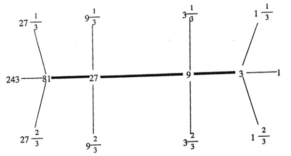
As $\Gamma_0(N) $ fixes $L_1 $ and $L_N $ it also fixes all lattices in the (N|1)-thread, that is all lattices occurring in a shortest path from $L_1 $ to $L_N $ (on the left a picture of the (200|1)-thread).

If $N=p_1^{a_1} p_2^{a_2} \ldots p_k^{a_k} $, then the (N|1)-thread has $2^k $ involutions as symmetries, called the Atkin-Lehner involutions. For every exact divisor $e || N $ (that is, $e|N $ and $gcd(e,\frac{N}{e})=1 $ we have an involution $W_e $ which acts by sending each point in the thread-cell corresponding to the prime divisors of $e $ to its antipodal cell-point and acts as the identity on the other prime-axes. For example, in the (200|1)-thread on the left, $W_8 $ is the left-right reflexion, $W_{25} $ the top-bottom reflexion and $W_{200} $ the antipodal reflexion. The set of all exact divisors of N becomes the group $~(\mathbb{Z}/2\mathbb{Z})^k $ under the operation $e \ast f = \frac{e \times f}{gcd(e,f)^2} $.

Most of the moonshine groups are of the form $\Gamma_0(n|h)+e,f,g,… $ for some $N=h.n $ such that $h | 24 $ and $h^2 | N $. The group $\Gamma_0(n|h) $ is then conjugate to the modular subgroup $\Gamma_0(\frac{n}{h}) $ by the element $\begin{bmatrix} h & 0 \ 0 & 1 \end{bmatrix} $. With $\Gamma_0(n|h)+e,f,g,… $ we mean that the group $\Gamma_0(n|h) $ is extended with the involutions $W_e,W_f,W_g,… $. If we simply add all Atkin-Lehner involutions we write $\Gamma_0(n|h)+ $ for the resulting group.

Finally, whenever $h \not= 1 $ there is a subgroup $\Gamma_0(n||h)+e,f,g,… $ which is the kernel of a character $\lambda $ being trivial on $\Gamma_0(N) $ and on all involutions $W_e $ for which every prime dividing $e $ also divides $\frac{n}{h} $, evaluating to $e^{\frac{2\pi i}{h}} $ on all cosets containing $\begin{bmatrix} 1 & \frac{1}{h} \ 0 & 1 \end{bmatrix} $ and to $e^{\pm \frac{2 \pi i }{h}} $ for cosets containing $\begin{bmatrix} 1 & 0 \ n & 0 \end{bmatrix} $ (with a + sign if $\begin{bmatrix} 0 & -1 \ N & 0 \end{bmatrix} $ is present and a – sign otherwise). Btw. it is not evident at all that this is a character, but hard work shows it is!

Clearly there are heavy restrictions on the numbers that actually occur in moonshine. In the paper On the discrete groups of moonshine, John Conway, John McKay and Abdellah Sebbar characterized the 171 arithmetic subgroups of $PSL_2(\mathbb{R}) $ occuring in monstrous moonshine as those of the form $G = \Gamma_0(n || h)+e,f,g,… $ which are

(a) of genus zero, meaning that the quotient of the upper-half plane by the action of $G \subset PSL_2(\mathbb{R}) $ by Moebius-transformations gives a Riemann surface of genus zero,
(b) the quotient group $G/\Gamma_0(nh) $ is a group of exponent 2 (generated by some Atkin-Lehner involutions), and
(c) every cusp can be mapped to $\infty $ by an element of $PSL_2(\mathbb{R}) $ which conjugates the group to one containing $\Gamma_0(nh) $.

Now, if $\Gamma_0(n || h)+e,f,g,… $ is of genus zero, so is the larger group $\Gamma_0(n | h)+e,f,g,… $, which in turn, is conjugated to the group $\Gamma_0(\frac{n}{h})+e,f,g,… $. Therefore, we need a list of all groups of the form $\Gamma_0(\frac{n}{h})+e,f,g,… $ which are of genus zero. There are exactly 123 of them, listed on the right.

How does this help to determine the structure of the p-subtree of the moonshine picture for the fifteen monster-primes p? Look for the largest p-power $p^k $ such that $p^k+e,f,g… $ appears in the list. That is for p=2,3,5,7,11,13,17,19,23,29,31,41,47,59,71 these powers are resp. 5,3,2,2,1,1,1,1,1,1,1,1,1,1,1. Next, look for the largest p-power $p^l $ dividing 24 (that is, 3 for p=2, 1 for p=3 and 0 for all other primes). Then, these relevant moonshine groups contain the modular subgroup $\Gamma_0(p^{k+2l}) $ and are contained in its normalizer in $PSL_2(\mathbb{R}) $ which by the Atkin-Lehner theorem is precisely the group $\Gamma_0(p^{k+l}|p^l)+ $.

Right, now the lattices fixed by $\Gamma_0(p^{k+2l}) $ (and permuted by its normalizer), that is the lattices in our p-subtree, are those that form the $~(p^{k+2l}|1) $-snake in Conway-speak. That is, the lattices whose hyper-distance to the $~(p^{k+l}|p^l) $-thread divides 24. So for all primes larger than 2 or 3, the p-tree is just the $~(p^l|1) $-thread.

For p=3 the 3-tree is the (243|1)-snake having the (81|3)-thread as its spine. It contains the following lattices, all of which are number-like.

Depicting the 2-tree, which is the (2048|1)-snake may take a bit longer… Perhaps someone should spend some time figuring out which cells of the product of these fifteen trees make up the moonshine picture!

Comments closed