Here a list of saved pdf-files of previous NeverEndingBooks-posts on geometry in reverse chronological order.
Leave a CommentTag: Riemann
After a lengthy spring-break, let us continue with our course on noncommutative geometry and $SL_2(\mathbb{Z}) $-representations. Last time, we have explained Grothendiecks mantra that all algebraic curves defined over number fields are contained in the profinite compactification
$\widehat{SL_2(\mathbb{Z})} = \underset{\leftarrow}{lim}~SL_2(\mathbb{Z})/N $ of the modular group $SL_2(\mathbb{Z}) $ and in the knowledge of a certain subgroup G of its group of outer automorphisms. In particular we have seen that many curves defined over the algebraic numbers $\overline{\mathbb{Q}} $ correspond to permutation representations of $SL_2(\mathbb{Z}) $. The profinite compactification $\widehat{SL_2}=\widehat{SL_2(\mathbb{Z})} $ is a continuous group, so it makes sense to consider its continuous n-dimensional representations $\mathbf{rep}_n^c~\widehat{SL_2} $ Such representations are known to have a finite image in $GL_n(\mathbb{C}) $ and therefore we get an embedding $\mathbf{rep}_n^c~\widehat{SL_2} \hookrightarrow \mathbf{rep}_n^{ss}~SL_n(\mathbb{C}) $ into all n-dimensional (semi-simple) representations of $SL_2(\mathbb{Z}) $. We consider such semi-simple points as classical objects as they are determined by – curves defined over $\overline{Q} $ – representations of (sporadic) finite groups – modlart data of fusion rings in RCTF – etc… To get a feel for the distinction between these continuous representations of the cofinite completion and all representations, consider the case of $\hat{\mathbb{Z}} = \underset{\leftarrow}{lim}~\mathbb{Z}/n \mathbb{Z} $. Its one-dimensional continuous representations are determined by roots of unity, whereas all one-dimensional (necessarily simple) representations of $\mathbb{Z}=C_{\infty} $ are determined by all elements of $\mathbb{C} $. Hence, the image of $\mathbf{rep}_1^c~\hat{\mathbb{Z}} \hookrightarrow \mathbf{rep}_1~C_{\infty} $ is contained in the unit circle
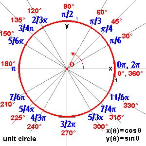
and though these points are very special there are enough of them (technically, they form a Zariski dense subset of all representations). Our aim will be twofold : (1) when viewing a classical object as a representation of $SL_2(\mathbb{Z}) $ we can define its modular content (which will be the noncommutative tangent space in this classical point to the noncommutative manifold of $SL_2(\mathbb{Z}) $). In this way we will associate noncommutative gadgets to our classical object (such as orders in central simple algebras, infinite dimensional Lie algebras, noncommutative potentials etc. etc.) which give us new tools to study these objects. (2) conversely, as we control the tangentspaces in these special points, they will allow us to determine other $SL_2(\mathbb{Z}) $-representations and as we vary over all classical objects, we hope to get ALL finite dimensional modular representations. I agree this may all sound rather vague, so let me give one example we will work out in full detail later on. Remember that one can reconstruct the sporadic simple Mathieu group $M_{24} $ from the dessin d’enfant
- This
- dessin determines a 24-dimensional permutation representation (of
- $M_{24} $ as well of $SL_2(\mathbb{Z}) $) which
- decomposes as the direct sum of the trivial representation and a simple
- 23-dimensional representation. We will see that the noncommutative
- tangent space in a semi-simple representation of
- $SL_2(\mathbb{Z}) $ is determined by a quiver (that is, an
- oriented graph) on as many vertices as there are non-isomorphic simple
- components. In this special case we get the quiver on two points
- $\xymatrix{\vtx{} \ar@/^2ex/[rr] & & \vtx{} \ar@/^2ex/[ll]
- \ar@{=>}@(ur,dr)^{96} } $ with just one arrow in each direction
- between the vertices and 96 loops in the second vertex. To the
- experienced tangent space-reader this picture (and in particular that
- there is a unique cycle between the two vertices) tells the remarkable
- fact that there is **a distinguished one-parameter family of
- 24-dimensional simple modular representations degenerating to the
- permutation representation of the largest Mathieu-group**. Phrased
- differently, there is a specific noncommutative modular Riemann surface
- associated to $M_{24} $, which is a new object (at least as far
- as I’m aware) associated to this most remarkable of sporadic groups.
- Conversely, from the matrix-representation of the 24-dimensional
- permutation representation of $M_{24} $ we obtain representants
- of all of this one-parameter family of simple
- $SL_2(\mathbb{Z}) $-representations to which we can then perform
- noncommutative flow-tricks to get a Zariski dense set of all
- 24-dimensional simples lying in the same component. (Btw. there are
- also such noncommutative Riemann surfaces associated to the other
- sporadic Mathieu groups, though not to the other sporadics…) So this
- is what we will be doing in the upcoming posts (10) : explain what a
- noncommutative tangent space is and what it has to do with quivers (11)
- what is the noncommutative manifold of $SL_2(\mathbb{Z}) $? and what is its connection with the Kontsevich-Soibelman coalgebra? (12)
- is there a noncommutative compactification of $SL_2(\mathbb{Z}) $? (and other arithmetical groups) (13) : how does one calculate the noncommutative curves associated to the Mathieu groups? (14) : whatever comes next… (if anything).
Today we will explain how curves defined over
$\overline{\mathbb{Q}} $ determine permutation representations
of the carthographic groups. We have seen that any smooth projective
curve $C $ (a Riemann surface) defined over the algebraic
closure $\overline{\mathbb{Q}} $ of the rationals, defines a
_Belyi map_ $\xymatrix{C \ar[rr]^{\pi} & & \mathbb{P}^1} $ which is only ramified over the three points
$\\{ 0,1,\infty \\} $. By this we mean that there are
exactly $d $ points of $C $ lying over any other point
of $\mathbb{P}^1 $ (we call $d $ the degree of
$\pi $) and that the number of points over $~0,1~ $ and
$~\infty $ is smaller than $~d $. To such a map we
associate a _dessin d\’enfant_, a drawing on $C $ linking the
pre-images of $~0 $ and $~1 $ with exactly $d $
edges (the preimages of the open unit-interval). Next, we look at
the preimages of $~0 $ and associate a permutation
$\tau_0 $ of $~d $ letters to it by cycling
counter-clockwise around these preimages and recording the edges we
meet. We repeat this procedure for the preimages of $~1 $ and
get another permutation $~\tau_1 $. That is, we obtain a
subgroup of the symmetric group $ \langle \tau_0,\tau_1
\rangle \subset S_d $ which is called the monodromy
group of the covering $\pi $.
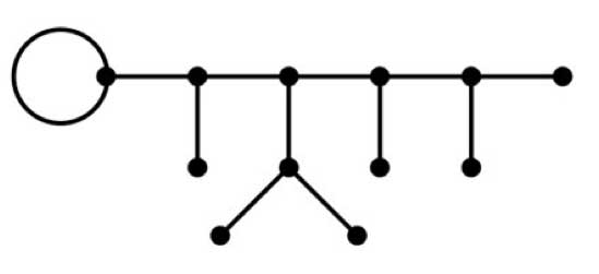
For example, the
dessin on the right is
associated to a degree $8 $ map $\mathbb{P}^1 \rightarrow
\mathbb{P}^1 $ and if we let the black (resp. starred) vertices be
the preimages of $~0 $ (respectively of $~1 $), then the
corresponding partitions are $\tau_0 = (2,3)(1,4,5,6) $
and $\tau_1 = (1,2,3)(5,7,8) $ and the monodromy group
is the alternating group $A_8 $ (use
GAP ).
But wait! The map is also
ramified in $\infty $ so why don\’t we record also a
permutation $\tau_{\infty} $ and are able to compute it from
the dessin? (Note that all three partitions are needed if we want to
reconstruct $C $ from the $~d $ sheets as they encode in
which order the sheets fit together around the preimages). Well,
the monodromy group of a $\mathbb{P}^1 $ covering ramified only
in three points is an epimorphic image of the fundamental
group of the sphere
minus three points $\pi_1(\mathbb{P}^1 – { 0,1,\infty
}) $ That is, the group of all loops beginning and
ending in a basepoint upto homotopy (that is, two such loops are the
same if they can be transformed into each other in a continuous way
while avoiding the three points).
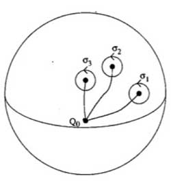 This group is generated by loops
$\sigma_i $ running from the basepoint to nearby the i-th
point, doing a counter-clockwise walk around it and going back to be
basepoint $Q_0 $ and the epimorphism to the monodromy group is given by sending
$\sigma_1 \mapsto \tau_0~\quad~\sigma_2 \mapsto
\tau_1~\quad~\sigma_3 \mapsto \tau_{\infty} $
Now,
these three generators are not independent. In fact, this fundamental
group is
$\pi_1(\mathbb{P}^1 – \\{ 0,1,\infty \\}) =
\langle \sigma_1,\sigma_2,\sigma_3~\mid~\sigma_1 \sigma_2
\sigma_3 = 1 \rangle $
 To understand this, let us begin
with an easier case, that of the sphere minus one point. The fundamental group of the plane minus one point is
$~\mathbb{Z} $ as it encodes how many times we walk around the
point. However, on the sphere the situation is different as we can make
our walk around the point longer and longer until the whole walk is done
at the backside of the sphere and then we can just contract our walk to
the basepoint. So, there is just one type of walk on a sphere minus one
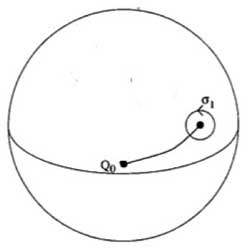
point (upto homotopy) whence this fundamental group is trivial. Next,
let us consider the sphere minus two points
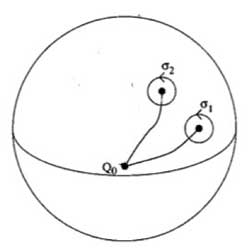
Repeat the foregoing to the walk $\sigma_2 $, that
is, strech the upper part of the circular tour all over the backside of
the sphere and then we see that we can move it to fit with the walk
$\sigma_1$ BUT for the orientation of the walk! That is, if we do this
modified walk $\sigma_1 \sigma_2^{\’} $ we just made the
trivial walk. So, this fundamental group is $\langle
\sigma_1,\sigma_2~\mid~\sigma_1 \sigma_2 = 1 \rangle =
\mathbb{Z} $ This is also the proof of the above claim. For,
we can modify the third walk $\sigma_3 $ continuously so that
it becomes the walk $\sigma_1 \sigma_2 $ but
with the reversed orientation ! As $\sigma_3 =
(\sigma_1 \sigma_2)^{-1} $ this allows us to compute the
\’missing\’ permutation $\tau_{\infty} = (\tau_0
\tau_1)^{-1} $ In the example above, we obtain
$\tau_{\infty}= (1,2,6,5,8,7,4)(3) $ so it has two cycles
corresponding to the fact that the dessin has two regions (remember we
should draw ths on the sphere) : the head and the outer-region. Hence,
the pre-images of $\infty$ correspond to the different regions of the
dessin on the curve $C $. For another example,
consider the degree 168 map
$K \rightarrow \mathbb{P}^1 $
which is the modified orbit map for the action of
$PSL_2(\mathbb{F}_7) $ on the Klein quartic.
The corresponding dessin is the heptagonal construction of the Klein
quartic
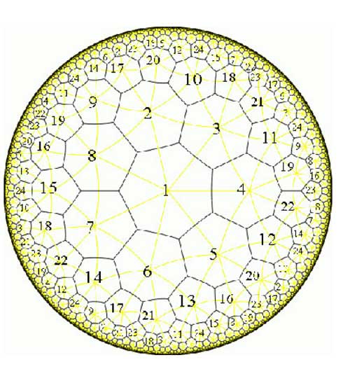
Here, the pre-images of 1 correspond to the midpoints of the
84 edges of the polytope whereas the pre-images of 0 correspond to the
56 vertices. We can label the 168 half-edges by numbers such that
$\tau_0 $ and $\tau_1 $ are the standard generators b
resp. a of the 168-dimensional regular representation (see the atlas
page ).
Calculating with GAP the element $\tau_{\infty} = (\tau_0
\tau_1)^{-1} = (ba)^{-1} $ one finds that this permutation
consists of 24 cycles of length 7, so again, the pre-images of
$\infty $ lie one in each of the 24 heptagonal regions of the
Klein quartic. Now, we are in a position to relate curves defined
over $\overline{Q} $ via their Belyi-maps and corresponding
dessins to Grothendiecks carthographic groups $\Gamma(2) $,
$\Gamma_0(2) $ and $SL_2(\mathbb{Z}) $. The
dessin gives a permutation representation of the monodromy group and
because the fundamental group of the sphere minus three
points $\pi_1(\mathbb{P}^1 – \\{ 0,1,\infty \\}) =
\langle \sigma_1,\sigma_2,\sigma_3~\mid~\sigma_1 \sigma_2
\sigma_3 = 1 \rangle = \langle \sigma_1,\sigma_2
\rangle $ is the free group op two generators, we see that
any dessin determines a permutation representation of the congruence
subgroup $\Gamma(2) $ (see this
post where we proved that this
group is free). A clean dessin is one for which one type of
vertex has all its valancies (the number of edges in the dessin meeting
the vertex) equal to one or two. (for example, the pre-images of 1 in
the Klein quartic-dessin or the pre-images of 1 in the monsieur Mathieu
example ) The corresponding
permutation $\tau_1 $ then consists of 2-cycles and hence the
monodromy group gives a permutation representation of the free
product $C_{\infty} \ast C_2 =
\Gamma_0(2) $ Finally, a clean dessin is said to be a
quilt dessin if also the other type of vertex has all its valancies
equal to one or three (as in the Klein quartic or Mathieu examples).
Then, the corresponding permutation has order 3 and for these
quilt-dessins the monodromy group gives a permutation representation of
the free product $C_2 \ast C_3 =
PSL_2(\mathbb{Z}) $ Next time we will see how this lead
Grothendieck to his anabelian geometric approach to the absolute Galois
group.