Yesterday, Jan Stienstra gave a talk at theARTS entitled “Quivers, superpotentials and Dimer Models”. He started off by telling that the talk was based on a paper he put on the arXiv Hypergeometric Systems in two Variables, Quivers, Dimers and Dessins d’Enfants but that he was not going to say a thing about dessins but would rather focuss on the connection with superpotentials instead…pleasing some members of the public, while driving others to utter despair.
Anyway, it gave me the opportunity to figure out for myself what dessins might have to do with dimers, whathever these beasts are. Soon enough he put on a slide containing the definition of a dimer and from that moment on I was lost in my own thoughts… realizing that a dessin d’enfant had to be a dimer for the Dedekind tessellation of its associated Riemann surface!
and a few minutes later I could slap myself on the head for not having thought of this before :
There is a natural way to associate to a Farey symbol (aka a permutation representation of the modular group) a quiver and a superpotential (aka a necklace) defining (conjecturally) a Calabi-Yau algebra! Moreover, different embeddings of the cuboid tree diagrams in the hyperbolic plane may (again conjecturally) give rise to all sorts of arty-farty fanshi-wanshi dualities…
I’ll give here the details of the simplest example I worked out during the talk and will come back to general procedure later, when I’ve done a reference check. I don’t claim any originality here and probably all of this is contained in Stienstra’s paper or in some physics-paper, so if you know of a reference, please leave a comment. Okay, remember the Dedekind tessellation ?
So, all hyperbolic triangles we will encounter below are colored black or white. Now, take a Farey symbol and consider its associated special polygon in the hyperbolic plane. If we start with the Farey symbol
[tex]\xymatrix{\infty \ar@{-}_{(1)}[r] & 0 \ar@{-}_{\bullet}[r] & 1 \ar@{-}_{(1)}[r] & \infty} [/tex]
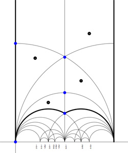 we get the special polygonal region bounded by the thick edges, the vertical edges are identified as are the two bottom edges. Hence, this fundamental domain has 6 vertices (the 5 blue dots and the point at $i \infty $) and 8 hyperbolic triangles (4 colored black, indicated by a black dot, and 4 white ones).
Right, now let us associate a quiver to this triangulation (which embeds the quiver in the corresponding Riemann surface). The vertices of the triangulation are also the vertices of the quiver (so in our case we are going for a quiver with 6 vertices). Every hyperbolic edge in the triangulation gives one arrow in the quiver between the corresponding vertices. The orientation of the arrow is determined by the color of a triangle of which it is an edge : if the triangle is black, we run around its edges counter-clockwise and if the triangle is white we run over its edges clockwise (that is, the orientation of the arrow is independent of the choice of triangles to determine it). In our example, there is one arrows directed from the vertex at $i $ to the vertex at $0 $, whether you use the black triangle on the left to determine the orientation or the white triangle on the right. If we do this for all edges in the triangulation we arrive at the quiver below
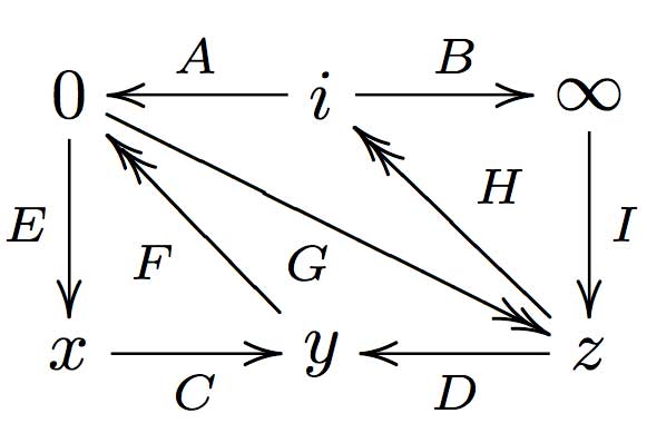
where x,y and z are the three finite vertices on the $\frac{1}{2} $-axis from bottom to top and where I’ve used the physics-convention for double arrows, that is there are two F-arrows, two G-arrows and two H-arrows. Observe that the quiver is of Calabi-Yau type meaning that there are as much arrows coming into a vertex as there are arrows leaving the vertex.
Now that we have our quiver we determine the superpotential as follows. Fix an orientation on the Riemann surface (for example counter-clockwise) and sum over all black triangles the product of the edge-arrows counterclockwise MINUS sum over all white triangles
the product of the edge arrows counterclockwise. So, in our example we have the cubic superpotential
$IH’B+HAG+G’DF+FEC-BHI-H’G’A-GFD-CEF’ $
From this we get the associated noncommutative algebra, which is the quotient of the path algebra of the above quiver modulo the following ‘commutativity relations’
$\begin{cases} GH &=G’H’ \\ IH’ &= IH \\ FE &= F’E \\ F’G’ &= FG \\ CF &= CF’ \\ EC &= GD \\ G’D &= EC \\ HA &= DF \\ DF’ &= H’A \\ AG &= BI \\ BI &= AG’ \end{cases} $
and morally this should be a Calabi-Yau algebra (( can someone who knows more about CYs verify this? )). This concludes the walk through of the procedure. Summarizing : to every Farey-symbol one associates a Calabi-Yau quiver and superpotential, possibly giving a Calabi-Yau algebra!
Leave a Comment Farey sequences have plenty of mysterious properties. For example, in 1924 J. Franel and
  Recall from
 Finally, identifying the red points (as they lie on geodesics connected to $\infty $ which are identified in the Farey code), adding even points on the remaining geodesics and numbering the obtained half-lines we obtain the dessin d’enfant given on the left hand side. To such a dessin we can associate its monodromy group which is a permutation group on the half-lines generated by an order two element indicating which half-lines make up a line and an order three element indicating which half-lines one encounters by walking counter-clockwise around a three-valent vertex. For the dessin on the left the group is therefore the subgroup of $S_{12} $ generated by the elements