Skip to content →

Tag: representations

Farey symbols of sporadic groups

John Conway once wrote :

There are almost as many different constructions of $M_{24} $ as there have been mathematicians interested in that most remarkable of all finite groups.

In the inguanodon post Ive added yet another construction of the Mathieu groups $M_{12} $ and $M_{24} $ starting from (half of) the Farey sequences and the associated cuboid tree diagram obtained by demanding that all edges are odd. In this way the Mathieu groups turned out to be part of a (conjecturally) infinite sequence of simple groups, starting as follows :

$L_2(7),M_{12},A_{16},M_{24},A_{28},A_{40},A_{48},A_{60},A_{68},A_{88},A_{96},A_{120},A_{132},A_{148},A_{164},A_{196},\ldots $

It is quite easy to show that none of the other sporadics will appear in this sequence via their known permutation representations. Still, several of the sporadic simple groups are generated by an element of order two and one of order three, so they are determined by a finite dimensional permutation representation of the modular group $PSL_2(\mathbb{Z}) $ and hence are hiding in a special polygonal region of the Dedekind’s tessellation

Let us try to figure out where the sporadic with the next simplest permutation representation is hiding : the second Janko group $J_2 $, via its 100-dimensional permutation representation. The Atlas tells us that the order two and three generators act as

e:= (1,84)(2,20)(3,48)(4,56)(5,82)(6,67)(7,55)(8,41)(9,35)(10,40)(11,78)(12, 100)(13,49)(14,37)(15,94)(16,76)(17,19)(18,44)(21,34)(22,85)(23,92)(24, 57)(25,75)(26,28)(27,64)(29,90)(30,97)(31,38)(32,68)(33,69)(36,53)(39,61) (42,73)(43,91)(45,86)(46,81)(47,89)(50,93)(51,96)(52,72)(54,74)(58,99) (59,95)(60,63)(62,83)(65,70)(66,88)(71,87)(77,98)(79,80);

v:= (1,80,22)(2,9,11)(3,53,87)(4,23,78)(5,51,18)(6,37,24)(8,27,60)(10,62,47) (12,65,31)(13,64,19)(14,61,52)(15,98,25)(16,73,32)(17,39,33)(20,97,58) (21,96,67)(26,93,99)(28,57,35)(29,71,55)(30,69,45)(34,86,82)(38,59,94) (40,43,91)(42,68,44)(46,85,89)(48,76,90)(49,92,77)(50,66,88)(54,95,56) (63,74,72)(70,81,75)(79,100,83);

But as the kfarey.sage package written by Chris Kurth calculates the Farey symbol using the L-R generators, we use GAP to find those

L = e*v^-1  and  R=e*v^-2 so

L=(1,84,22,46,70,12,79)(2,58,93,88,50,26,35)(3,90,55,7,71,53,36)(4,95,38,65,75,98,92)(5,86,69,39,14,6,96)(8,41,60,72,61,17, 64)(9,57,37,52,74,56,78)(10,91,40,47,85,80,83)(11,23,49,19,33,30,20)(13,77,15,59,54,63,27)(16,48,87,29,76,32,42)(18,68, 73,44,51,21,82)(24,28,99,97,45,34,67)(25,81,89,62,100,31,94)

R=(1,84,80,100,65,81,85)(2,97,69,17,13,92,78)(3,76,73,68,16,90,71)(4,54,72,14,24,35,11)(5,34,96,18,42,32,44)(6,21,86,30,58, 26,57)(7,29,48,53,36,87,55)(8,41,27,19,39,52,63)(9,28,93,66,50,99,20)(10,43,40,62,79,22,89)(12,83,47,46,75,15,38)(23,77, 25,70,31,59,56)(33,45,82,51,67,37,61)(49,64,60,74,95,94,98)

Defining these permutations in sage and using kfarey, this gives us the Farey-symbol of the associated permutation representation

L=SymmetricGroup(Integer(100))("(1,84,22,46,70,12,79)(2,58,93,88,50,26,35)(3,90,55,7,71,53,36)(4,95,38,65,75,98,92)(5,86,69,39,14,6,96)(8,41,60,72,61,17, 64)(9,57,37,52,74,56,78)(10,91,40,47,85,80,83)(11,23,49,19,33,30,20)(13,77,15,59,54,63,27)(16,48,87,29,76,32,42)(18,68, 73,44,51,21,82)(24,28,99,97,45,34,67)(25,81,89,62,100,31,94)")

R=SymmetricGroup(Integer(100))("(1,84,80,100,65,81,85)(2,97,69,17,13,92,78)(3,76,73,68,16,90,71)(4,54,72,14,24,35,11)(5,34,96,18,42,32,44)(6,21,86,30,58, 26,57)(7,29,48,53,36,87,55)(8,41,27,19,39,52,63)(9,28,93,66,50,99,20)(10,43,40,62,79,22,89)(12,83,47,46,75,15,38)(23,77, 25,70,31,59,56)(33,45,82,51,67,37,61)(49,64,60,74,95,94,98)")

sage: FareySymbol("Perm",[L,R])

[[0, 1, 4, 3, 2, 5, 18, 13, 21, 71, 121, 413, 292, 463, 171, 50, 29, 8, 27, 46, 65, 19, 30, 11, 3, 10, 37, 64, 27, 17, 7, 4, 5], [1, 1, 3, 2, 1, 2, 7, 5, 8, 27, 46, 157, 111, 176, 65, 19, 11, 3, 10, 17, 24, 7, 11, 4, 1, 3, 11, 19, 8, 5, 2, 1, 1], [-3, 1, 4, 4, 2, 3, 6, -3, 7, 13, 14, 15, -3, -3, 15, 14, 11, 8, 8, 10, 12, 12, 10, 9, 5, 5, 9, 11, 13, 7, 6, 3, 2, 1]]

Here, the first string gives the numerators of the cusps, the second the denominators and the third gives the pairing information (where [tex[-2 $ denotes an even edge and $-3 $ an odd edge. Fortunately, kfarey also allows us to draw the special polygonal region determined by a Farey-symbol. So, here it is (without the pairing data) :

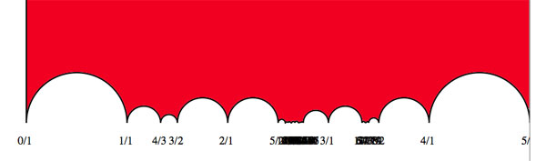
the hiding place of $J_2 $…

It would be nice to have (a) other Farey-symbols associated to the second Janko group, hopefully showing a pattern that one can extend into an infinite family as in the inguanodon series and (b) to determine Farey-symbols of more sporadic groups.

Leave a Comment

KMS, Gibbs & zeta function

Time to wrap up this series on the Bost-Connes algebra. Here’s what we have learned so far : the convolution product on double cosets

$\begin{bmatrix} 1 & \mathbb{Z} \\ 0 & 1 \end{bmatrix} \backslash \begin{bmatrix} 1 & \mathbb{Q} \\ 0 & \mathbb{Q}_{> 0} \end{bmatrix} / \begin{bmatrix} 1 & \mathbb{Z} \\ 0 & 1 \end{bmatrix} $

is a noncommutative algebra, the Bost-Connes Hecke algebra $\mathcal{H} $, which is a bi-chrystalline graded algebra (somewhat weaker than ‘strongly graded’) with part of degree one the group-algebra $\mathbb{Q}[\mathbb{Q}/\mathbb{Z}] $. Further, $\mathcal{H} $ has a natural one-parameter family of algebra automorphisms $\sigma_t $ defined by $\sigma_t(X_n) = n^{it}X_n $ and $\sigma_t(Y_{\lambda})=Y_{\lambda} $.

For any algebra $A $ together with a one-parameter family of automorphisms $\sigma_t $ one is interested in KMS-states or Kubo-Martin-Schwinger states with parameter $\beta $, $KMS_{\beta} $ (this parameter is often called the ‘invers temperature’ of the system) as these are suitable equilibria states. Recall that a state is a special linear functional $\phi $ on $A $ (in particular it must have norm one) and it belongs to $KMS_{\beta} $ if the following commutation relation holds for all elements $a,b \in A $

$\phi(a \sigma_{i\beta}(b)) = \phi(b a) $

Let us work out the special case when $A $ is the matrix-algebra $M_n(\mathbb{C}) $. To begin, all algebra-automorphisms are inner in this case, so any one-parameter family of automorphisms is of the form

$\sigma_t(a) = e^{itH} a e^{-itH} $

where $e^{itH} $ is the matrix-exponential of the nxn matrix $H $. For any parameter $\beta $ we claim that the linear functional

$\phi(a) = \frac{1}{tr(e^{-\beta H})} tr(a e^{-\beta H}) $

is a KMS-state.Indeed, we have for all matrices $a,b \in M_n(\mathbb{C}) $ that

$\phi(a \sigma_{i \beta}(b)) = \frac{1}{tr(e^{-\beta H})} tr(a e^{- \beta H} b e^{\beta H} e^{- \beta H}) $

$= \frac{1}{tr(e^{-\beta H})} tr(a e^{-\beta H} b) = \frac{1}{tr(e^{-\beta H})} tr(ba e^{-\beta H}) = \phi(ba) $

(the next to last equality follows from cyclic-invariance of the trace map).
These states are usually called Gibbs states and the normalization factor $\frac{1}{tr(e^{-\beta H})} $ (needed because a state must have norm one) is called the partition function of the system. Gibbs states have arisen from the study of ideal gases and the place to read up on all of this are the first two chapters of the second volume of “Operator algebras and quantum statistical mechanics” by Ola Bratelli and Derek Robinson.

This gives us a method to construct KMS-states for an arbitrary algebra $A $ with one-parameter automorphisms $\sigma_t $ : take a simple n-dimensional representation $\pi~:~A \mapsto M_n(\mathbb{C}) $, find the matrix $H $ determining the image of the automorphisms $\pi(\sigma_t) $ and take the Gibbs states as defined before.

Let us return now to the Bost-Connes algebra $\mathcal{H} $. We don’t know any finite dimensional simple representations of $\mathcal{H} $ but, sure enough, have plenty of graded simple representations. By the usual strongly-graded-yoga they should correspond to simple finite dimensional representations of the part of degree one $\mathbb{Q}[\mathbb{Q}/\mathbb{Z}] $ (all of them being one-dimensional and corresponding to characters of $\mathbb{Q}/\mathbb{Z} $).

Hence, for any $u \in \mathcal{G} = \prod_p \hat{\mathbb{Z}}_p^{\ast} $ (details) we have a graded simple $\mathcal{H} $-representation $S_u = \oplus_{n \in \mathbb{N}_+} \mathbb{C} e_n $ with action defined by

$\begin{cases} \pi_u(X_n)(e_m) = e_{nm} \\ \pi_u(Y_{\lambda})(e_m) = e^{2\pi i n u . \lambda} e_m \end{cases} $

Here, $u.\lambda $ is computed using the ‘chinese-remainder-identification’ $\mathcal{A}/\mathcal{R} = \mathbb{Q}/\mathbb{Z} $ (details).

Even when the representations $S_u $ are not finite dimensional, we can mimic the above strategy : we should find a linear operator $H $ determining the images of the automorphisms $\pi_u(\sigma_t) $. We claim that the operator is defined by $H(e_n) = log(n) e_n $ for all $n \in \mathbb{N}_+ $. That is, we claim that for elements $a \in \mathcal{H} $ we have

$\pi_u(\sigma_t(a)) = e^{itH} \pi_u(a) e^{-itH} $

So let us compute the action of both sides on $e_m $ when $a=X_n $. The left hand side gives $\pi_u(n^{it}X_n)(e_m) = n^{it} e_{mn} $ whereas the right-hand side becomes

$e^{itH}\pi_u(X_n) e^{-itH}(e_m) = e^{itH} \pi_u(X_n) m^{-it} e_m = $

$e^{itH} m^{-it} e_{mn} = (mn)^{it} m^{-it} e_{mn} = n^{it} e_{mn} $

proving the claim. For any parameter $\beta $ this then gives us a KMS-state for the Bost-Connes algebra by

$\phi_u(a) = \frac{1}{Tr(e^{-\beta H})} Tr(\pi_u(a) e^{-\beta H}) $

Finally, let us calculate the normalization factor (or partition function) $\frac{1}{Tr(e^{-\beta H})} $. Because $e^{-\beta H}(e_n) = n^{-\beta} e_n $ we have for that the trace

$Tr(e^{-\beta H}) = \sum_{n \in \mathbb{N}_+} \frac{1}{n^{\beta}} = \zeta(\beta) $

is equal to the Riemann zeta-value $\zeta(\beta) $ (at least when $\beta > 1 $).

Summarizing, we started with the definition of the Bost-Connes algebra $\mathcal{H} $, found a canonical one-parameter subgroup of algebra automorphisms $\sigma_t $ and computed that the natural equilibria states with respect to this ‘time evolution’ have as their partition function the Riemann zeta-function. Voila!

Leave a Comment

abc on adelic Bost-Connes

The adelic interpretation of the Bost-Connes Hecke algebra $\mathcal{H} $ is based on three facts we’ve learned so far :

  1. The diagonal embedding of the rational numbers $\delta~:~\mathbb{Q} \rightarrow \prod_p \mathbb{Q}_p $ has its image in the adele ring $\mathcal{A} $. ( details )

  2. There is an exact sequence of semigroups $1 \rightarrow \mathcal{G} \rightarrow \mathcal{I} \cap \mathcal{R} \rightarrow \mathbb{N}^+_{\times} \rightarrow 1 $ where $\mathcal{I} $ is the idele group, that is the units of $\mathcal{A} $, where $\mathcal{R} = \prod_p \mathbb{Z}_p $ and where $\mathcal{G} $ is the group (!) $\prod_p \mathbb{Z}_p^* $. ( details )

  3. There is an isomorphism of additive groups $\mathbb{Q}/\mathbb{Z} \simeq \mathcal{A}/\mathcal{R} $. ( details )

Because $\mathcal{R} $ is a ring we have that $a\mathcal{R} \subset \mathcal{R} $ for any $a=(a_p)_p \in \mathcal{I} \cap \mathcal{R} $. Therefore, we have an induced ‘multiplication by $a $’ morphism on the additive group $\mathcal{A}/\mathcal{R} \rightarrow^{a.} \mathcal{A}/\mathcal{R} $ which is an epimorphism for all $a \in \mathcal{I} \cap \mathcal{R} $.

In fact, it is easy to see that the equation $a.x = y $ for $y \in \mathcal{A}/\mathcal{R} $ has precisely $n_a = \prod_p p^{d(a)} $ solutions. In particular, for any $a \in \mathcal{G} = \prod_p \mathbb{Z}_p^* $, multiplication by $a $ is an isomorphism on $\mathcal{A}/\mathcal{R} = \mathbb{Q}/\mathbb{Z} $.

But then, we can form the crystalline semigroup graded skew-group algebra $\mathbb{Q}(\mathbb{Q}/\mathbb{Z}) \bowtie (\mathcal{I} \cap \mathcal{R}) $. It is the graded vectorspace $\oplus_{a \in \mathcal{I} \cap \mathcal{R}} X_a \mathbb{Q}[\mathbb{Q}/\mathbb{Z}] $ with commutation relation
$Y_{\lambda}X_a = X_a Y_{a \lambda} $ for the base-vectors $Y_{\lambda} $ with $\lambda \in \mathbb{Q}/\mathbb{Z} $. Recall from last time we need to use approximation (or the Chinese remainder theorem) to determine the class of $a \lambda $ in $\mathbb{Q}/\mathbb{Z} $.

We can also extend it to a bi-crystalline graded algebra because multiplication by $a \in \mathcal{I} \cap \mathcal{R} $ has a left-inverse which determines the commutation relations $Y_{\lambda} X_a^* = X_a^* (\frac{1}{n_a})(\sum_{a.\mu = \lambda} Y_{\mu}) $. Let us call this bi-crystalline graded algebra $\mathcal{H}_{big} $, then we have the following facts

  1. For every $a \in \mathcal{G} $, the element $X_a $ is a unit in $\mathcal{H}_{big} $ and $X_a^{-1}=X_a^* $. Conjugation by $X_a $ induces on the subalgebra $\mathbb{Q}[\mathbb{Q}/\mathbb{Z}] $ the map $Y_{\lambda} \rightarrow Y_{a \lambda} $.

  2. Using the diagonal embedding $\delta $ restricted to $\mathbb{N}^+_{\times} $ we get an embedding of algebras $\mathcal{H} \subset \mathcal{H}_{big} $ and conjugation by $X_a $ for any $a \in \mathcal{G} $ sends $\mathcal{H} $ to itself. However, as the $X_a \notin \mathcal{H} $, the induced automorphisms are now outer!

Summarizing : the Bost-Connes Hecke algebra $\mathcal{H} $ encodes a lot of number-theoretic information :

  • the additive structure is encoded in the sub-algebra which is the group-algebra $\mathbb{Q}[\mathbb{Q}/\mathbb{Z}] $
  • the multiplicative structure in encoded in the epimorphisms given by multiplication with a positive natural number (the commutation relation with the $X_m $
  • the automorphism group of $\mathbb{Q}/\mathbb{Z} $ extends to outer automorphisms of $\mathcal{H} $

That is, the Bost-Connes algebra can be seen as a giant mashup of number-theory of $\mathbb{Q} $. So, if one can prove something specific about this algebra, it is bound to have interesting number-theoretic consequences.

But how will we study $\mathcal{H} $? Well, the bi-crystalline structure of it tells us that $\mathcal{H} $ is a ‘good’-graded algebra with part of degree one the group-algebra $\mathbb{Q}[\mathbb{Q}/\mathbb{Z}] $. This group-algebra is a formally smooth algebra and we study such algebras by studying their finite dimensional representations.

Hence, we should study ‘good’-graded formally smooth algebras (such as $\mathcal{H} $) by looking at their graded representations. This will then lead us to Connes’ “fabulous states”…

Leave a Comment