representations – Page 20 – neverendingbooks

sexing up curves

Published June 10, 2005 by lieven

Here the
story of an idea to construct new examples of non-commutative compact
manifolds, the computational difficulties one runs into and, when they
are solved, the white noise one gets. But, perhaps, someone else can
spot a gem among all gibberish…
[Qurves](https://lievenlb.local/toolkit/pdffile.php?pdf=/TheLibrary/papers/qaq.pdf) (aka quasi-free algebras, aka formally smooth
algebras) are the \’affine\’ pieces of non-commutative manifolds. Basic
examples of qurves are : semi-simple algebras (e.g. group algebras of
finite groups), [path algebras of
quivers](http://www.lns.cornell.edu/spr/2001-06/msg0033251.html) and
coordinate rings of affine smooth curves. So, let us start with an
affine smooth curve $X$ and spice it up to get a very non-commutative
qurve. First, we bring in finite groups. Let $G$ be a finite group
acting on $X$ , then we can form the skew-group algebra $A = \mathbfk [X] ★ G$ . These are examples of prime Noetherian qurves (aka
hereditary orders). A more pompous way to phrase this is that these are
precisely the [one-dimensional smooth Deligne-Mumford
stacks](http://www.math.lsa.umich.edu/~danielch/paper/stacks.pdf).
As the 21-st century will turn out to be the time we discovered the
importance of non-Noetherian algebras, let us make a jump into the
wilderness and consider the amalgamated free algebra product $A = (k [X] ★ G) *_{k G} \mathbfk H$ where $G \subset H$ is an interesting extension of finite groups. Then, $A$ is
again a qurve on which $H$ acts in a way compatible with the $G$ -action
on $X$ and $A$ is hugely non-commutative… A very basic example :
let $Z / 2 Z$ act on the affine line $\mathbfk [x]$ by
sending $x \mapsto - x$ and consider a finite [simple
group](http://mathworld.wolfram.com/SimpleGroup.html) $M$ . As every
simple group has an involution, we have an embedding
$Z / 2 Z \subset M$ and can construct the qurve
$A = (\mathbfk [x] ★ Z / 2 Z) *_{\mathbfk Z / 2 Z} \mathbfk M$ on which the simple group $M$ acts
compatible with the involution on the affine line. To study the
corresponding non-commutative manifold, that is the Abelian category
$rep A$ of all finite dimensional representations of $A$ we have
to compute the [one quiver to rule them
all](https://lievenlb.local/master/coursenotes/onequiver.pdf) for
$A$ . Because $A$ is a qurve, all its representation varieties
${rep}_{n} A$ are smooth affine varieties, but they may have several
connected components. The direct sum of representations turns the set of
all these components into an Abelian semigroup and the vertices of the
\’one quiver\’ correspond to the generators of this semigroup whereas
the number of arrows between two such generators is given by the
dimension of $E x t_{A}^{1} (S_{i}, S_{j})$ where $S_{i}, S_{j}$ are simple
$A$ -representations lying in the respective components. All this
may seem hard to compute but it can be reduced to the study of another
quiver, the Zariski quiver associated to $A$ which is a bipartite quiver
with on the left the \’one quiver\’ for $\mathbfk [x] ★ Z / 2 Z$ which is just $Misplaced &$ (where the two vertices
correspond to the two simples of $Z / 2 Z$ ) and on the
right the \’one quiver\’ for $k M$ (which just consists of as
many verticers as there are simple representations for $M$ ) and where
the number of arrows from a left- to a right-vertex is the number of
$Z / 2 Z$ -morphisms between the respective simples. To
make matters even more concrete, let us consider the easiest example
when $M = A_{5}$ the alternating group on $5$ letters. The corresponding
Zariski quiver then turns out to be $Misplaced &$ The Euler-form of this quiver can then be used to
calculate the dimensions of the EXt-spaces giving the number of arrows
in the \’one quiver\’ for $A$ . To find the vertices, that is, the
generators of the component semigroup we have to find the minimal
integral solutions to the pair of equations saying that the number of
simple $Z / 2 Z$ components based on the left-vertices is
equal to that one the right-vertices. In this case it is easy to see
that there are as many generators as simple $M$ representations. For
$A_{5}$ they correspond to the dimension vectors (for the Zariski quiver
having the first two components on the left) ${\begin{cases} (1, 2, 0, 0, 0, 0, 1) \\ (1, 2, 0, 0, 0, 1, 0) \\ (3, 2, 0, 0, 1, 0, 0) \\ (2, 2, 0, 1, 0, 0, 0) \\ (1, 0, 1, 0, 0, 0, 0) \end{cases}$ We now have all
info to determine the \’one quiver\’ for $A$ and one would expect a nice
result. Instead one obtains a complete graph on all vertices with plenty
of arrows. More precisely one obtains as the one quiver for $A_{5}$
$Misplaced &$
with the number of arrows (in each direction) indicated. Not very
illuminating, I find. Still, as the one quiver is symmetric it follows
that all quotient varieties ${iss}_{n} A$ have a local Poisson
structure. Clearly, the above method can be generalized easily and all
examples I did compute so far have this \’nearly complete graph\’
feature. One might hope that if one would start with very special
curves and groups, one might obtain something more interesting. Another
time I\’ll tell what I got starting from Klein\’s quartic (on which the
simple group $P S L_{2} (F_{7})$ acts) when the situation was sexed-up
to the sporadic simple Mathieu group $M_{24}$ (of which
$P S L_{2} (F_{7})$ is a maximal subgroup).

back

Published June 9, 2005 by lieven

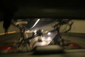
If you recognize where this picture was
taken, you will know that I\’m back from France. If you look closer you
will see two bikes, my own Bulls mountainbike
in front and Stijn\’s
lightweight bike behind.
If you see the relative position of the
saddles, you will know that Stijn is at least 20 cm taller. Let me add
that he is also at least 20 yrs. younger and 20 kgs. stronger and it
will be clear that I had a hard (but fun) time trying to follow him
uphill. Btw. this picture (and the next dozen or so) was taken by Jan and I\’ll try to add the next
days a couple of shots he likes more.

Since then I\’ve been
writing up a paper which I hope will be ready to put online by
september. It\’s all about using non-commutative geometry to construct
representations of arithmetic groups, a bit like the Granada Notes but with a dash of
Double Poisson
Algebras to it.

A positive outcome of this short break is
a renewed interest in the NeverEndingBooks project, but more on this
later. For now, let me just add that Raf
decided to feed my noncommutative geometry@n (version 2)
to a printing on demand publisher. So, if you want a perfect bound
paperback version of it (for 12 Euro approx.) you\’d better email him at once (at the
moment he will order just 5 copies).

why nag? (3)

Published March 29, 2005 by lieven

Here is
the construction of this normal space or chart $\mathbf{chart}_{\Gamma}$ . The sub-semigroup of $Z^5$ (all
dimension vectors of Q) consisting of those vectors $\alpha=(a_1,a_2,b_1,b_2,b_3)$ satisfying the numerical condition $a_1+a_2=n=b_1+b_2+b_3$ is generated by six dimension vectors,
namely those of the 6 non-isomorphic one-dimensional solutions in $\mathbf{rep}~\Gamma$

$S_1 = \xymatrix@=.4cm{ & & & & \vtx{1} \\ \vtx{1} \ar[rrrru]^1 \ar[rrrrd] \ar[rrrrddd] & & & & \\ & & & & \vtx{0} \\ \vtx{0} \ar[rrrruuu] \ar[rrrru] \ar[rrrrd] & & & & \\ & & & & \vtx{0}} \qquad S_2 = \xymatrix@=.4cm{ & & & & \vtx{0} \\ \vtx{0} \ar[rrrru] \ar[rrrrd] \ar[rrrrddd] & & & & \\& & & & \vtx{1} \\\vtx{1} \ar[rrrruuu] \ar[rrrru]^1 \ar[rrrrd] & & & & \\ & & & & \vtx{0}}$

$S_3 = \xymatrix@=.4cm{ & & & & \vtx{0} \\ \vtx{1} \ar[rrrru] \ar[rrrrd] \ar[rrrrddd]^1 & & & & \\ & & & & \vtx{0} \\ \vtx{0} \ar[rrrruuu] \ar[rrrru] \ar[rrrrd] & & & & \\ & & & & \vtx{1}} \qquad S_4 = \xymatrix@=.4cm{ & & & & \vtx{1} \\ \vtx{0} \ar[rrrru] \ar[rrrrd] \ar[rrrrddd] & & & & \\ & & & & \vtx{0} \\ \vtx{1} \ar[rrrruuu]^1 \ar[rrrru] \ar[rrrrd] & & & & \\ & & & & \vtx{0}}$

$S_5 = \xymatrix@=.4cm{ & & & & \vtx{0} \\ \vtx{1} \ar[rrrru] \ar[rrrrd]^1 \ar[rrrrddd] & & & & \\ & & & & \vtx{1} \\ \vtx{0} \ar[rrrruuu] \ar[rrrru] \ar[rrrrd] & & & & \\ & & & & \vtx{0}} \qquad S_6 = \xymatrix@=.4cm{ & & & & \vtx{0} \\ \vtx{0} \ar[rrrru] \ar[rrrrd] \ar[rrrrddd] & & & & \\ & & & & \vtx{0} \\ \vtx{1} \ar[rrrruuu] \ar[rrrru] \ar[rrrrd]^1 & & & & \\ & & & & \vtx{1}}$

In
particular, in any component $\mathbf{rep}_{\alpha}~Q$ containing an open subset of
representations corresponding to solutions in $\mathbf{rep}~\Gamma$ we have a particular semi-simple solution

$M = S_1^{\oplus g_1} \oplus S_2^{\oplus g_2} \oplus S_3^{\oplus g_3} \oplus S_4^{\oplus g_4} \oplus S_5^{\oplus g_5} \oplus S_6^{\oplus g_6}$

and in
particular $\alpha = (g_1+g_3+g_5,g_2+g_4+g_6,g_1+g_4,g_2+g_5,g_3+g_6)$ . The normal space
to the $GL(\alpha)$ -orbit of M in $\mathbf{rep}_{\alpha}~Q$ can be identified with the representation
space $\mathbf{rep}_{\beta}~Q$ where $\beta=(g_1,\ldots,g_6)$ and Q is the quiver of the following
form

$\xymatrix{ & \vtx{g_1} \ar@/^/[ld]^{C_{16}} \ar@/^/[rd]^{C_{12}} & \\ \vtx{g_6} \ar@/^/[ru]^{C_{61}} \ar@/^/[d]^{C_{65}} & & \vtx{g_2} \ar@/^/[lu]^{C_{21}} \ar@/^/[d]^{C_{23}} \\ \vtx{g_5} \ar@/^/[u]^{C_{56}} \ar@/^/[rd]^{C_{54}} & & \vtx{g_3} \ar@/^/[u]^{C_{32}} \ar@/^/[ld]^{C_{34}} \\ & \vtx{g_4} \ar@/^/[lu]^{C_{45}} \ar@/^/[ru]^{C_{43}} & }$

and we can
even identify how the small matrices $C_{ij}$ fit
into the $3 \times 2$ block-decomposition of the base-change matrix B

$B = \begin{bmatrix} \begin{array}{ccc|ccc} 1_{a_1} & 0 & 0 & C_{21} & 0 & C_{61} \\ 0 & C_{34} & C_{54} & 0 & 1_{a_4} & 0 \\ \hline C_{12} & C_{32} & 0 & 1_{a_2} & 0 & 0 \\ 0 & 0 & 1_{a_5} & 0 & C_{45} & C_{65} \\ \hline 0 & 1_{a_3} & 0 & C_{23} & C_{43} & 0 \\ C_{16} & 0 & C_{56} & 0 & 0 & 1_{a_6} \\ \end{array} \end{bmatrix}$

Hence, it makes sense
to call Q the non-commutative normal space to the isomorphism problem in
$\mathbf{rep}~\Gamma$ . Moreover, under this correspondence simple
representations of Q (for which both the dimension vectors and
distinguishing characters are known explicitly) correspond to simple
solutions in $\mathbf{rep}~\Gamma$ .

Having completed our promised
approach via non-commutative geometry to the classification problem of
solutions to the braid relation, it is time to collect what we have
learned. Let $\beta=(g_1,\ldots,g_6)$ with $n = \gamma_1 + \ldots + \gamma_6$ , then for every
non-zero scalar $\lambda \in \mathbb{C}^*$ the matrices

$X = \lambda B^{-1} \begin{bmatrix} 1_{g_1+g_4} & 0 & 0 \\ 0 & \rho^2 1_{g_2+g_5} & 0 \\ 0 & 0 & \rho 1_{g_3+g_6} \end{bmatrix} B \begin{bmatrix} 1_{g_1+g_3+g_5} & 0 \\ 0 & -1_{g_2+g_4+g_6} \end{bmatrix}$

$Y = \lambda \begin{bmatrix} 1_{g_1+g_3+g_5} & 0 \\ 0 & -1_{g_2+g_4+g_6} \end{bmatrix} B^{-1} \begin{bmatrix} 1_{g_1+g_4} & 0 & 0 \\ 0 & \rho^2 1_{g_2+g_5} & 0 \\ 0 & 0 & \rho 1_{g_3+g_6} \end{bmatrix} B$

give a solution of size
n to the braid relation. Moreover, such a solution can be simple only if
the following numerical relations are satisfied

$g_i \leq g_{i-1} + g_{i+1}$

where indices are viewed
modulo 6. In fact, if these conditions are satisfied then a sufficiently
general representation of Q does determine a simple solution in $\mathbf{rep}~B_3$ and conversely, any sufficiently general simple n
size solution of the braid relation can be conjugated to one of the
above form. Here, by sufficiently general we mean a Zariski open (hence
dense) subset.

That is, for all integers n we have constructed
nearly all (meaning a dense subset) simple solutions to the braid
relation. As to the classification problem, if we have representants of
simple $\beta$ -dimensional representations of the quiver Q, then the corresponding
solutions $(X,Y)$ of
the braid relation represent different orbits (up to finite overlap
coming from the fact that our linearizations only give an analytic
isomorphism, or in algebraic terms, an etale map). Such representants
can be constructed for low dimensional $\beta$ .
Finally, our approach also indicates why the classification of
braid-relation solutions of size $\leq 5$ is
easier : from size 6 on there are new classes of simple
Q-representations given by going round the whole six-cycle!

Tag: representations

sexing up curves

back

why nag? (3)