 Last time we have
seen that the noncommutative manifold of a Riemann surface can be viewed
as that Riemann surface together with a loop in each point. The extra
loop-structure tells us that all finite dimensional representations of
the coordinate ring can be found by separating over points and those
living at just one point are classified by the isoclasses of nilpotent
matrices, that is are parametrized by the partitions (corresponding
to the sizes of the Jordan blocks). In addition, these loops tell us
that the Riemann surface locally looks like a Riemann sphere, so an
equivalent mental picture of the local structure of this
noncommutative manifold is given by the picture on teh left, where the surface is part of the Riemann surface
and a sphere is placed at every point. Today we will consider
genuine noncommutative curves and describe their corresponding
noncommutative manifolds.
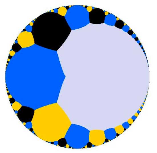
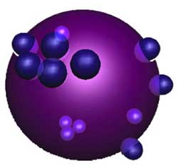 Here, a mental picture of such a
_noncommutative sphere_ to keep in mind would be something
like the picture on the right. That is, in most points of the sphere we place as before again
a Riemann sphere but in a finite number of points a different phenomen
occurs : we get a cluster of infinitesimally nearby points. We
will explain this picture with an easy example. Consider the
complex plane $\mathbb{C} $, the points of which are just the
one-dimensional representations of the polynomial algebra in one
variable $\mathbb{C}[z] $ (any algebra map $\mathbb{C}[z] \rightarrow \mathbb{C} $ is fully determined by the image of z). On this plane we
have an automorphism of order two sending a complex number z to its
negative -z (so this automorphism can be seen as a point-reflexion
with center the zero element 0). This automorphism extends to
the polynomial algebra, again induced by sending z to -z. That
is, the image of a polynomial $f(z) \in \mathbb{C}[z] $ under this
automorphism is f(-z).
With this data we can form a noncommutative
algebra, the _skew-group algebra_ $\mathbb{C}[z] \ast C_2 $ the
elements of which are either of the form $f(z) \ast e $ or $g(z) \ast g $ where
$C_2 = \langle g : g^2=e \rangle $ is the cyclic group of order two
generated by the automorphism g and f(z),g(z) are arbitrary
polynomials in z.
The multiplication on this algebra is determined by
the following rules
$(g(z) \ast g)(f(z) \ast e) = g(z)f(-z) \astg $ whereas $(f(z) \ast e)(g(z) \ast g) = f(z)g(z) \ast g $
$(f(z) \ast e)(g(z) \ast e) = f(z)g(z) \ast e $ whereas $(f(z) \ast g)(g(z)\ast g) = f(z)g(-z) \ast e $
That is, multiplication in the
$\mathbb{C}[z] $ factor is the usual multiplication, multiplication in
the $C_2 $ factor is the usual group-multiplication but when we want
to get a polynomial from right to left over a group-element we have to
apply the corresponding automorphism to the polynomial (thats why we
call it a _skew_ group-algebra).
Alternatively, remark that as
a $\mathbb{C} $-algebra the skew-group algebra $\mathbb{C}[z] \ast C_2 $ is
an algebra with unit element 1 = 1\aste and is generated by
the elements $X = z \ast e $ and $Y = 1 \ast g $ and that the defining
relations of the multiplication are
$Y^2 = 1 $ and $Y.X =-X.Y $
hence another description would
be
$\mathbb{C}[z] \ast C_2 = \frac{\mathbb{C} \langle X,Y \rangle}{ (Y^2-1,XY+YX) } $
It can be shown that skew-group
algebras over the coordinate ring of smooth curves are _noncommutative
smooth algebras_ whence there is a noncommutative manifold associated
to them. Recall from last time the noncommutative manifold of a
smooth algebra A is a device to classify all finite dimensional
representations of A upto isomorphism Let us therefore try to
determine some of these representations, starting with the
one-dimensional ones, that is, algebra maps from
$\mathbb{C}[z] \ast C_2 = \frac{\mathbb{C} \langle X,Y \rangle}{ (Y^2-1,XY+YX) } \rightarrow \mathbb{C} $
Such a map is determined by the image of X and that of
Y. Now, as $Y^2=1 $ we have just two choices for the image of Y
namely +1 or -1. But then, as the image is a commutative algebra
and as XY+YX=0 we must have that the image of 2XY is zero whence the
image of X must be zero. That is, we have only
two one-dimensional representations, namely $S_+ : X \rightarrow 0, Y \rightarrow 1 $
and $S_- : X \rightarrow 0, Y \rightarrow -1 $
This is odd! Can
it be that our noncommutative manifold has just 2 points? Of course not.
In fact, these two points are the exceptional ones giving us a cluster
of nearby points (see below) whereas most points of our
noncommutative manifold will correspond to 2-dimensional
representations!
So, let’s hunt them down. The
center of $\mathbb{C}[z]\ast C_2 $ (that is, the elements commuting with
all others) consists of all elements of the form $f(z)\ast e $ with f an
_even_ polynomial, that is, f(z)=f(-z) (because it has to commute
with 1\ast g), so is equal to the subalgebra $\mathbb{C}[z^2]\ast e $.
The
manifold corresponding to this subring is again the complex plane
$\mathbb{C} $ of which the points correspond to all one-dimensional
representations of $\mathbb{C}[z^2]\ast e $ (determined by the image of
$z^2\ast e $).
We will now show that to each point of $\mathbb{C} – { 0 } $
corresponds a simple 2-dimensional representation of
$\mathbb{C}[z]\ast C_2 $.
If a is not zero, we will consider the
quotient of the skew-group algebra modulo the twosided ideal generated
by $z^2\ast e-a $. It turns out
that
$\frac{\mathbb{C}[z]\ast C_2}{(z^2\aste-a)} =
\frac{\mathbb{C}[z]}{(z^2-a)} \ast C_2 = (\frac{\mathbb{C}[z]}{(z-\sqrt{a})}
\oplus \frac{\mathbb{C}[z]}{(z+\sqrt{a})}) \ast C_2 = (\mathbb{C}
\oplus \mathbb{C}) \ast C_2 $
where the skew-group algebra on the
right is given by the automorphism g on $\mathbb{C} \oplus \mathbb{C} $ interchanging the two factors. If you want to
become more familiar with working in skew-group algebras work out the
details of the fact that there is an algebra-isomorphism between
$(\mathbb{C} \oplus \mathbb{C}) \ast C_2 $ and the algebra of $2 \times 2 $ matrices $M_2(\mathbb{C}) $. Here is the
identification
$~(1,0)\aste \rightarrow \begin{bmatrix} 1 & 0 \\ 0 & 0 \end{bmatrix} $
$~(0,1)\aste \rightarrow \begin{bmatrix} 0 & 0 \\ 0 & 1 \end{bmatrix} $
$~(1,0)\astg \rightarrow \begin{bmatrix} 0 & 1 \\ 0 & 0 \end{bmatrix} $
$~(0,1)\astg \rightarrow \begin{bmatrix} 0 & 0 \\ 1 & 0 \end{bmatrix} $
so you have to verify that multiplication
on the left hand side (that is in $(\mathbb{C} \oplus \mathbb{C}) \ast
C_2 $) coincides with matrix-multiplication of the associated
matrices.
Okay, this begins to look like what we are after. To
every point of the complex plane minus zero (or to every point of the
Riemann sphere minus the two points ${ 0,\infty } $) we have
associated a two-dimensional simple representation of the skew-group
algebra (btw. simple means that the matrices determined by the images
of X and Y generate the whole matrix-algebra).
In fact, we
now have already classified ‘most’ of the finite dimensional
representations of $\mathbb{C}[z]\ast C_2 $, namely those n-dimensional
representations
$\mathbb{C}[z]\ast C_2 =
\frac{\mathbb{C} \langle X,Y \rangle}{(Y^2-1,XY+YX)} \rightarrow M_n(\mathbb{C}) $
for which the image of X is an invertible $n \times n $ matrix. We can show that such representations only exist when
n is an even number, say n=2m and that any such representation is
again determined by the geometric/combinatorial data we found last time
for a Riemann surface.
That is, It is determined by a finite
number ${ P_1,\dots,P_k } $ of points from $\mathbb{C} – 0 $ where
k is at most m. For each index i we have a positive
number $a_i $ such that $a_1+\dots+a_k=m $ and finally for each i we
also have a partition of $a_i $.
That is our noncommutative
manifold looks like all points of $\mathbb{C}-0 $ with one loop in each
point. However, we have to remember that each point now determines a
simple 2-dimensional representation and that in order to get all
finite dimensional representations with det(X) non-zero we have to
scale up representations of $\mathbb{C}[z^2] $ by a factor two.
The technical term here is that of a Morita equivalence (or that the
noncommutative algebra is an Azumaya algebra over
$\mathbb{C}-0 $).
What about the remaining representations, that
is, those for which Det(X)=0? We have already seen that there are two
1-dimensional representations $S_+ $ and $S_- $ lying over 0, so how
do they fit in our noncommutative manifold? Should we consider them as
two points and draw also a loop in each of them or do we have to do
something different? Rememer that drawing a loop means in our
geometry -> representation dictionary that the representations
living at that point are classified in the same way as nilpotent
matrices.
Hence, drawing a loop in $S_+ $ would mean that we have a
2-dimensional representation of $\mathbb{C}[z]\ast C_2 $ (different from
$S_+ \oplus S_+ $) and any such representation must correspond to
matrices
$X \rightarrow \begin{bmatrix} 0 & 1 \\ 0 & 0 \end{bmatrix} $ and $Y \rightarrow \begin{bmatrix} 1 & 0 \\ 0 & 1 \end{bmatrix} $
But this is not possible as these matrices do
_not_ satisfy the relation XY+YX=0. Hence, there is no loop in $S_+ $
and similarly also no loop in $S_- $.
However, there are non
semi-simple two dimensional representations build out of the simples
$S_+ $ and $S_- $. For, consider the matrices
$X \rightarrow \begin{bmatrix} 0 & 1 \\ 0 & 0 \end{bmatrix} $ and $Y \rightarrow \begin{bmatrix} 1 & 0 \\ 0 & -1 \end{bmatrix} $
then these
matrices _do_ satisfy XY+YX=0! (and there is another matrix-pair
interchanging $\pm 1 $ in the Y-matrix). In erudite terminology this
says that there is a _nontrivial extension_ between $S_+ $ and $S_- $
and one between $S_- $ and $S_+ $.
In our dictionary we will encode this
information by the picture
$\xymatrix{\vtx{}
\ar@/^2ex/[rr] & & \vtx{} \ar@/^2ex/[ll]} $
where the two
vertices correspond to the points $S_+ $ and $S_- $ and the arrows
represent the observed extensions. In fact, this data suffices to finish
our classification project of finite dimensional representations of
the noncommutative curve $\mathbb{C}[z] \ast C_2 $.
Those with Det(X)=0
are of the form : $R \oplus T $ where R is a representation with
invertible X-matrix (which we classified before) and T is a direct
sum of representations involving only the simple factors $S_+ $ and
$S_- $ and obtained by iterating the 2-dimensional idea. That is, for
each factor the Y-matrix has alternating $\pm 1 $ along the diagonal
and the X-matrix is the full nilpotent Jordan-matrix.
So
here is our picture of the noncommutative manifold of the
noncommutative curve $\mathbb{C}[z]\ast C_2 $ : the points are all points
of $\mathbb{C}-0 $ together with one loop in each of them together
with two points lying over 0 where we draw the above picture of arrows
between them. One should view these two points as lying
infinetesimally close to each other and the gluing
data
$\xymatrix{\vtx{} \ar@/^2ex/[rr] & & \vtx{}
\ar@/^2ex/[ll]} $
contains enough information to determine
that all other points of the noncommutative manifold in the vicinity of
this cluster should be two dimensional simples! The methods used
in this simple minded example are strong enough to determine the
structure of the noncommutative manifold of _any_ noncommutative curve.
So, let us look at a real-life example. Once again, take the
Kleinian quartic In a previous
course-post we recalled that
there is an action by automorphisms on the Klein quartic K by the
finite simple group $PSL_2(\mathbb{F}_7) $ of order 168. Hence, we
can form the noncommutative Klein-quartic $K \ast PSL_2(\mathbb{F}_7) $
(take affine pieces consisting of complements of orbits and do the
skew-group algebra construction on them and then glue these pieces
together again).
We have also seen that the orbits are classified
under a Belyi-map $K \rightarrow \mathbb{P}^1_{\mathbb{C}} $ and that this map
had the property that over any point of $\mathbb{P}^1_{\mathbb{C}}
– { 0,1,\infty } $ there is an orbit consisting of 168 points
whereas over 0 (resp. 1 and $\infty $) there is an orbit
consisting of 56 (resp. 84 and 24 points).
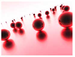
So what is
the noncommutative manifold associated to the noncommutative Kleinian?
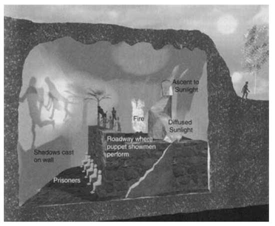
Well, it looks like the picture we had at the start of this
post For all but three points of the Riemann sphere
$\mathbb{P}^1 – { 0,1,\infty } $ we have one point and one loop
(corresponding to a simple 168-dimensional representation of $K \ast
PSL_2(\mathbb{F}_7) $) together with clusters of infinitesimally nearby
points lying over 0,1 and $\infty $ (the cluster over 0
is depicted, the two others only indicated).
Over 0 we have
three points connected by the diagram
$\xymatrix{& \vtx{} \ar[ddl] & \\ & & \\ \vtx{} \ar[rr] & & \vtx{} \ar[uul]} $
where each of the vertices corresponds to a
simple 56-dimensional representation. Over 1 we have a cluster of
two points corresponding to 84-dimensional simples and connected by
the picture we had in the $\mathbb{C}[z]\ast C_2 $ example).
Finally,
over $\infty $ we have the most interesting cluster, consisting of the
seven dwarfs (each corresponding to a simple representation of dimension
24) and connected to each other via the
picture
$\xymatrix{& & \vtx{} \ar[dll] & & \\ \vtx{} \ar[d] & & & & \vtx{} \ar[ull] \\ \vtx{} \ar[dr] & & & & \vtx{} \ar[u] \\ & \vtx{} \ar[rr] & & \vtx{} \ar[ur] &} $
Again, this noncommutative manifold gives us
all information needed to give a complete classification of all finite
dimensional $K \ast PSL_2(\mathbb{F}_7) $-representations. One
can prove that all exceptional clusters of points for a noncommutative
curve are connected by a cyclic quiver as the ones above. However, these
examples are still pretty tame (in more than one sense) as these
noncommutative algebras are finite over their centers, are Noetherian
etc. The situation will become a lot wilder when we come to exotic
situations such as the noncommutative manifold of
$SL_2(\mathbb{Z}) $…