 Mumford’s drawing has a clear emphasis on the vertical direction. The set of all vertical lines corresponds to taking the fibers of the natural ‘structural morphism’ : $\pi~:~\mathbf{spec}(\mathbb{Z}[t]) \rightarrow \mathbf{spec}(\mathbb{Z}) $ coming from the inclusion $\mathbb{Z} \subset \mathbb{Z}[t] $. That is, we consider the intersection $P \cap \mathbb{Z} $ of a prime ideal $P \subset \mathbb{Z}[t] $ with the subring of constants.
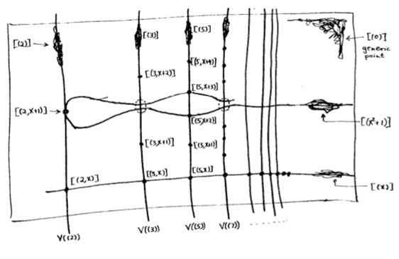
Two options arise : either $P \cap \mathbb{Z} \not= 0 $, in which case the intersection is a principal prime ideal $~(p) $ for some prime number $p $ (and hence $P $ itself is bigger or equal to $p\mathbb{Z}[t] $ whence its geometric object is contained in the vertical line $\mathbb{V}((p)) $, the fiber $\pi^{-1}((p)) $ of the structural morphism over $~(p) $), or, the intersection $P \cap \mathbb{Z}[t] = 0 $ reduces to the zero ideal (in which case the extended prime ideal $P \mathbb{Q}[x] = (q(x)) $ is a principal ideal of the rational polynomial algebra $\mathbb{Q}[x] $, and hence the geometric object corresponding to $P $ is a horizontal curve in Mumford’s drawing, or is the whole arithmetic plane itself if $P=0 $).
Because we know already that any ‘point’ in Mumford’s drawing corresponds to a maximal ideal of the form $\mathfrak{m}=(p,f(x)) $ (see last time), we see that every point lies on precisely one of the set of all vertical coordinate axes corresponding to the prime numbers ${~\mathbb{V}((p)) = \mathbf{spec}(\mathbb{F}_p[x]) = \pi^{-1}((p))~} $. In particular, two different vertical lines do not intersect (or, in ringtheoretic lingo, the ‘vertical’ prime ideals $p\mathbb{Z}[x] $ and $q\mathbb{Z}[x] $ are comaximal for different prime numbers $p \not= q $).
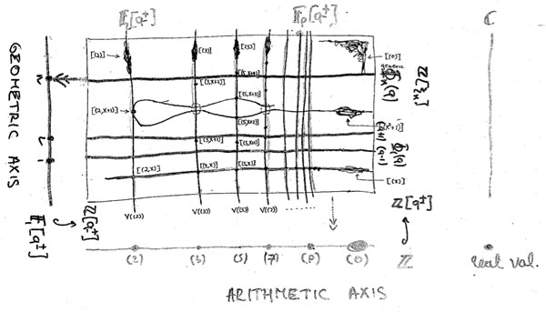
That is, the structural morphism is a projection onto the “arithmetic axis” (which is $\mathbf{spec}(\mathbb{Z}) $) and we get the above picture. The extra vertical line to the right of the picture is there because in arithmetic geometry it is customary to include also the archimedean valuations and hence to consider the ‘compactification’ of the arithmetic axis $\mathbf{spec}(\mathbb{Z}) $ which is $\overline{\mathbf{spec}(\mathbb{Z})} = \mathbf{spec}(\mathbb{Z}) \cup { v_{\mathbb{R}} } $.
 Yuri I. Manin is advocating for years the point that we should take the terminology ‘arithmetic surface’ for $\mathbf{spec}(\mathbb{Z}[x]) $ a lot more seriously. That is, there ought to be, apart from the projection onto the ‘z-axis’ (that is, the arithmetic axis $\mathbf{spec}(\mathbb{Z}) $) also a projection onto the ‘x-axis’ which he calls the ‘geometric axis’.
But then, what are the ‘points’ of this geometric axis and what are their fibers under this second projection?
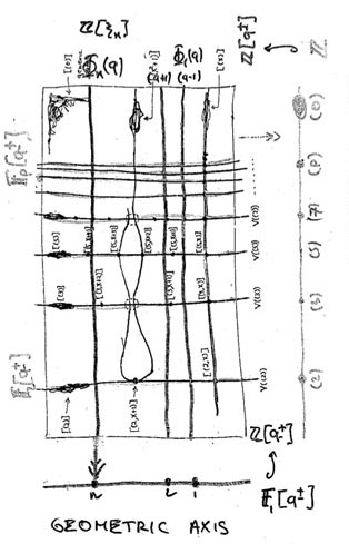
We have seen above that the vertical coordinate line over the prime number $~(p) $ coincides with $\mathbf{spec}(\mathbb{F}_p[x]) $, the affine line over the finite field $\mathbb{F}_p $. But all of these different lines, for varying primes $p $, should project down onto the same geometric axis. Manin’s idea was to take therefore as the geometric axis the affine line $\mathbf{spec}(\mathbb{F}_1[x]) $, over the virtual field with one element, which should be thought of as being the limit of the finite fields $\mathbb{F}_p $ when $p $ goes to one!
How many points does $\mathbf{spec}(\mathbb{F}_1[x]) $ have? Over a virtual object one can postulate whatever one wants and hope for an a posteriori explanation. $\mathbb{F}_1 $-gurus tell us that there should be exactly one point of size n on the affine line over $\mathbb{F}_1 $, corresponding to the unique degree n field extension $\mathbb{F}_{1^n} $. However, it is difficult to explain this from the limiting perspective…
Over a genuine finite field $\mathbb{F}_p $, the number of points of thickness $n $ (that is, those for which the residue field is isomorphic to the degree n extension $\mathbb{F}_{p^n} $) is equal to the number of monic irreducible polynomials of degree n over $\mathbb{F}_p $. This number is known to be $\frac{1}{n} \sum_{d | n} \mu(\frac{n}{d}) p^d $ where $\mu(k) $ is the Moebius function. But then, the limiting number should be $\frac{1}{n} \sum_{d | n} \mu(\frac{n}{d}) = \delta_{n1} $, that is, there can only be one point of size one…
Alternatively, one might consider the zeta function counting the number $N_n $ of ideals having a quotient consisting of precisely $p^n $ elements. Then, we have for genuine finite fields $\mathbb{F}_p $ that $\zeta(\mathbb{F}_p[x]) = \sum_{n=0}^{\infty} N_n t^n = 1 + p t + p^2 t^2 + p^3 t^3 + \ldots $, whence in the limit it should become
$1+t+t^2 +t^3 + \ldots $ and there is exactly one ideal in $\mathbb{F}_1[x] $ having a quotient of cardinality n and one argues that this unique quotient should be the unique point with residue field $\mathbb{F}_{1^n} $ (though it might make more sense to view this as the unique n-fold extension of the unique size-one point $\mathbb{F}_1 $ corresponding to the quotient $\mathbb{F}_1[x]/(x^n) $…)
A perhaps more convincing reasoning goes as follows. If $\overline{\mathbb{F}_p} $ is an algebraic closure of the finite field $\mathbb{F}_p $, then the points of the affine line over $\overline{\mathbb{F}_p} $ are in one-to-one correspondence with the maximal ideals of $\overline{\mathbb{F}_p}[x] $ which are all of the form $~(x-\lambda) $ for $\lambda \in \overline{\mathbb{F}_p} $. Hence, we get the points of the affine line over the basefield $\mathbb{F}_p $ as the orbits of points over the algebraic closure under the action of the Galois group $Gal(\overline{\mathbb{F}_p}/\mathbb{F}_p) $.
‘Common wisdom’ has it that one should identify the algebraic closure of the field with one element $\overline{\mathbb{F}_{1}} $ with the group of all roots of unity $\mathbb{\mu}_{\infty} $ and the corresponding Galois group $Gal(\overline{\mathbb{F}_{1}}/\mathbb{F}_1) $ as being generated by the power-maps $\lambda \rightarrow \lambda^n $ on the roots of unity. But then there is exactly one orbit of length n given by the n-th roots of unity $\mathbb{\mu}_n $, so there should be exactly one point of thickness n in $\mathbf{spec}(\mathbb{F}_1[x]) $ and we should then identity the corresponding residue field as $\mathbb{F}_{1^n} = \mathbb{\mu}_n $.
Whatever convinces you, let us assume that we can identify the non-generic points of $\mathbf{spec}(\mathbb{F}_1[x]) $ with the set of positive natural numbers ${ 1,2,3,\ldots } $ with $n $ denoting the unique size n point with residue field $\mathbb{F}_{1^n} $. Then, what are the fibers of the projection onto the geometric axis $\phi~:~\mathbf{spec}(\mathbb{Z}[x]) \rightarrow \mathbf{spec}(\mathbb{F}_1[x]) = { 1,2,3,\ldots } $?
These fibers should correspond to ‘horizontal’ principal prime ideals of $\mathbb{Z}[x] $. Manin proposes to consider $\phi^{-1}(n) = \mathbb{V}((\Phi_n(x))) $ where $\Phi_n(x) $ is the n-th cyclotomic polynomial. The nice thing about this proposal is that all closed points of $\mathbf{spec}(\mathbb{Z}[x]) $ lie on one of these fibers!
Indeed, the residue field at such a point (corresponding to a maximal ideal $\mathfrak{m}=(p,f(x)) $) is the finite field $\mathbb{F}_{p^n} $ and as all its elements are either zero or an $p^n-1 $-th root of unity, it does lie on the curve determined by $\Phi_{p^n-1}(x) $.
As a consequence, the localization $\mathbb{Z}[x]_{cycl} $ of the integral polynomial ring $\mathbb{Z}[x] $ at the multiplicative system generated by all cyclotomic polynomials is a principal ideal domain (as all height two primes evaporate in the localization), and, the fiber over the generic point of $\mathbf{spec}(\mathbb{F}_1[x]) $ is $\mathbf{spec}(\mathbb{Z}[x]_{cycl}) $, which should be compared to the fact that the fiber of the generic point in the projection onto the arithmetic axis is $\mathbf{spec}(\mathbb{Q}[x]) $ and $\mathbb{Q}[x] $ is the localization of $\mathbb{Z}[x] $ at the multiplicative system generated by all prime numbers).
Hence, both the vertical coordinate lines and the horizontal ‘lines’ contain all closed points of the arithmetic plane. Further, any such closed point $\mathfrak{m}=(p,f(x)) $ lies on the intersection of a vertical line $\mathbb{V}((p)) $ and a horizontal one $\mathbb{V}((\Phi_{p^n-1}(x))) $ (if $deg(f(x))=n $).
That is, these horizontal and vertical lines form a coordinate system, at least for the closed points of $\mathbf{spec}(\mathbb{Z}[x]) $.
Still, there is a noticeable difference between the two sets of coordinate lines. The vertical lines do not intersect meaning that $p\mathbb{Z}[x]+q\mathbb{Z}[x]=\mathbb{Z}[x] $ for different prime numbers p and q. However, in general the principal prime ideals corresponding to the horizontal lines $~(\Phi_n(x)) $ and $~(\Phi_m(x)) $ are not comaximal when $n \not= m $, that is, these ‘lines’ may have points in common! This will lead to an exotic new topology on the roots of unity… (to be continued).
Comments closed
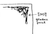 The doodle in the right upper corner depicts the
 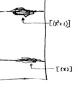 Let’s move over to the doodles in the lower right-hand corner. They represent the geometric object corresponding to principal prime ideals of the form $~(p(x)) $, where $p(x) $ in an
 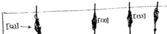 Apart from these ‘horizontal’ curves, there are also ‘vertical’ lines corresponding to the principal prime ideals $~(p) $, containing the polynomials, all of which coefficients are divisible by the prime number $p $. These are indeed prime ideals of $\mathbb{Z}[x] $, because their quotients are
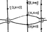 Right! So far we managed to depict the zero prime ideal (the whole plane) and the principal prime ideals of $\mathbb{Z}[x] $ (the horizontal curves and the vertical lines). Remains to depict the