Tag: geometry

On2 : transfinite number hacking

Published January 8, 2009 by lieven

In ONAG, John Conway proves that the symmetric version of his recursive definition of addition and multiplcation on the surreal numbers make the class On of all Cantor’s ordinal numbers into an algebraically closed Field of characteristic two : On2 (pronounced ‘Onto’), and, in particular, he identifies a subfield
with the algebraic closure of the field of two elements. What makes all of this somewhat confusing is that Cantor had already defined a (badly behaving) addition, multiplication and exponentiation on ordinal numbers.

Over the last week I’ve been playing a bit with sage to prove a few exotic identities involving ordinal numbers. Here’s one of them ($\omega $ is the first infinite ordinal number, that is, $\omega={ 0,1,2,\ldots } $),

$~(\omega^{\omega^{13}})^{47} = \omega^{\omega^7} + 1 $

answering a question in Hendrik Lenstra’s paper Nim multiplication.

However, it will take us a couple of posts before we get there. Let’s begin by trying to explain what brought this on. On september 24th 2008 there was a meeting, intended for a general public, called a la rencontre des dechiffeurs, celebrating the 50th birthday of the IHES.

One of the speakers was Alain Connes and the official title of his talk was “L’ange de la géométrie, le diable de l’algèbre et le corps à un élément” (the angel of geometry, the devil of algebra and the field with one element). Instead, he talked about a seemingly trivial problem : what is the algebraic closure of $\mathbb{F}_2 $, the field with two elements? My only information about the actual content of the talk comes from the following YouTube-blurb

Alain argues that we do not have a satisfactory description of $\overline{\mathbb{F}}_2 $, the algebraic closure of $\mathbb{F}_2 $. Naturally, it is the union (or rather, limit) of all finite fields $\mathbb{F}_{2^n} $, but, there are too many non-canonical choices to make here.

Recall that $\mathbb{F}_{2^k} $ is a subfield of $\mathbb{F}_{2^l} $ if and only if $k $ is a divisor of $l $ and so we would have to take the direct limit over the integers with respect to the divisibility relation… Of course, we can replace this by an increasing sequence of a selection of cofinal fields such as

$\mathbb{F}_{2^{1!}} \subset \mathbb{F}_{2^{2!}} \subset \mathbb{F}_{2^{3!}} \subset \ldots $

But then, there are several such suitable sequences! Another ambiguity comes from the description of $\mathbb{F}_{2^n} $. Clearly it is of the form $\mathbb{F}_2[x]/(f(x)) $ where $f(x) $ is a monic irreducible polynomial of degree $n $, but again, there are several such polynomials. An attempt to make a canonical choice of polynomial is to take the ‘first’ suitable one with respect to some natural ordering on the polynomials. This leads to the so called Conway polynomials.

Conway polynomials for the prime $2 $ have only been determined up to degree 400-something, so in the increasing sequence above we would already be stuck at the sixth term $\mathbb{F}_{2^{6!}} $…

So, what Alain Connes sets as a problem is to find another, more canonical, description of $\overline{\mathbb{F}}_2 $. The problem is not without real-life interest as most finite fields appearing in cryptography or coding theory are subfields of $\overline{\mathbb{F}}_2 $.

(My guess is that Alain originally wanted to talk about the action of the Galois group on the roots of unity, which would be the corresponding problem over the field with one element and would explain the title of the talk, but decided against it. If anyone knows what ‘coupling-problem’ he is referring to, please drop a comment.)

Surely, Connes is aware of the fact that there exists a nice canonical recursive construction of $\overline{\mathbb{F}}_2 $ due to John Conway, using Georg Cantor’s ordinal numbers.

In fact, in chapter 6 of his book On Numbers And Games, John Conway proves that the symmetric version of his recursive definition of addition and multiplcation on the surreal numbers make the class $\mathbf{On} $ of all Cantor’s ordinal numbers into an algebraically closed Field of characteristic two : $\mathbf{On}_2 $ (pronounced ‘Onto’), and, in particular, he identifies a subfield

$\overline{\mathbb{F}}_2 \simeq [ \omega^{\omega^{\omega}} ] $

with the algebraic closure of $\mathbb{F}_2 $. What makes all of this somewhat confusing is that Cantor had already defined a (badly behaving) addition, multiplication and exponentiation on ordinal numbers. To distinguish between the Cantor/Conway arithmetics, Conway (and later Lenstra) adopt the convention that any expression between square brackets refers to Cantor-arithmetic and un-squared ones to Conway’s. So, in the description of the algebraic closure just given $[ \omega^{\omega^{\omega}} ] $ is the ordinal defined by Cantor-exponentiation, whereas the exotic identity we started out with refers to Conway’s arithmetic on ordinal numbers.

Let’s recall briefly Cantor’s ordinal arithmetic. An ordinal number $\alpha $ is the order-type of a totally ordered set, that is, if there is an order preserving bijection between two totally ordered sets then they have the same ordinal number (or you might view $\alpha $ itself as a totally ordered set, namely the set of all strictly smaller ordinal numbers, so e.g. $0= \emptyset,1= { 0 },2={ 0,1 },\ldots $).

For two ordinals $\alpha $ and $\beta $, the addition $[\alpha + \beta ] $ is the order-type of the totally ordered set $\alpha \sqcup \beta $ (the disjoint union) ordered compatible with the total orders in $\alpha $ and $\beta $ and such that every element of $\beta $ is strictly greater than any element from $\alpha $. Observe that this definition depends on the order of the two factors. For example,$ [1 + \omega] = \omega $ as there is an order preserving bijection ${ \tilde{0},0,1,2,\ldots } \rightarrow { 0,1,2,3,\ldots } $ by $\tilde{0} \mapsto 0,n \mapsto n+1 $. However, $\omega \not= [\omega + 1] $ as there can be no order preserving bijection ${ 0,1,2,\ldots } \rightarrow { 0,1,2,\ldots,0_{max} } $ as the first set has no maximal element whereas the second one does. So, Cantor’s addition has the bad property that it may be that $[\alpha + \beta] \not= [\beta + \alpha] $.

The Cantor-multiplication $ \alpha . \beta $ is the order-type of the product-set $\alpha \times \beta $ ordered via the last differing coordinate. Again, this product has the bad property that it may happen that $[\alpha . \beta] \not= [\beta . \alpha] $ (for example $[2 . \omega ] \not=[ \omega . 2 ] $). Finally, the exponential $\beta^{\alpha} $ is the order type of the set of all maps $f~:~\alpha \rightarrow \beta $ such that $f(a) \not=0 $ for only finitely many $a \in \alpha $, and ordered via the last differing function-value.

Cantor’s arithmetic allows normal-forms for ordinal numbers. More precisely, with respect to any ordinal number $\gamma \geq 2 $, every ordinal number $\alpha \geq 1 $ has a unique expression as

$\alpha = [ \gamma^{\alpha_0}.\eta_0 + \gamma^{\alpha_1}.\eta_1 + \ldots + \gamma^{\alpha_m}.\eta_m] $

for some natural number $m $ and such that $\alpha \geq \alpha_0 > \alpha_1 > \ldots > \alpha_m \geq 0 $ and all $1 \leq \eta_i < \gamma $. In particular, taking the special cases $\gamma = 2 $ and $\gamma = \omega $, we have the following two canonical forms for any ordinal number $\alpha $

$[ 2^{\alpha_0} + 2^{\alpha_1} + \ldots + 2^{\alpha_m}] = \alpha = [ \omega^{\beta_0}.n_0 + \omega^{\beta_1}.n_1 + \ldots + \omega^{\beta_k}.n_k] $

with $m,k,n_i $ natural numbers and $\alpha \geq \alpha_0 > \alpha_1 > \ldots > \alpha_m \geq 0 $ and $\alpha \geq \beta_0 > \beta_1 > \ldots > \beta_k \geq 0 $. Both canonical forms will be important when we consider the (better behaved) Conway-arithmetic on $\mathbf{On}_2 $, next time.

One Comment

Manin’s geometric axis

Published December 23, 2008 by lieven

Mumford’s drawing has a clear emphasis on the vertical direction. The set of all vertical lines corresponds to taking the fibers of the natural ‘structural morphism’ : $\pi~:~\mathbf{spec}(\mathbb{Z}[t]) \rightarrow \mathbf{spec}(\mathbb{Z}) $ coming from the inclusion $\mathbb{Z} \subset \mathbb{Z}[t] $. That is, we consider the intersection $P \cap \mathbb{Z} $ of a prime ideal $P \subset \mathbb{Z}[t] $ with the subring of constants.

Two options arise : either $P \cap \mathbb{Z} \not= 0 $, in which case the intersection is a principal prime ideal $~(p) $ for some prime number $p $ (and hence $P $ itself is bigger or equal to $p\mathbb{Z}[t] $ whence its geometric object is contained in the vertical line $\mathbb{V}((p)) $, the fiber $\pi^{-1}((p)) $ of the structural morphism over $~(p) $), or, the intersection $P \cap \mathbb{Z}[t] = 0 $ reduces to the zero ideal (in which case the extended prime ideal $P \mathbb{Q}[x] = (q(x)) $ is a principal ideal of the rational polynomial algebra $\mathbb{Q}[x] $, and hence the geometric object corresponding to $P $ is a horizontal curve in Mumford’s drawing, or is the whole arithmetic plane itself if $P=0 $).

Because we know already that any ‘point’ in Mumford’s drawing corresponds to a maximal ideal of the form $\mathfrak{m}=(p,f(x)) $ (see last time), we see that every point lies on precisely one of the set of all vertical coordinate axes corresponding to the prime numbers ${~\mathbb{V}((p)) = \mathbf{spec}(\mathbb{F}_p[x]) = \pi^{-1}((p))~} $. In particular, two different vertical lines do not intersect (or, in ringtheoretic lingo, the ‘vertical’ prime ideals $p\mathbb{Z}[x] $ and $q\mathbb{Z}[x] $ are comaximal for different prime numbers $p \not= q $).

That is, the structural morphism is a projection onto the “arithmetic axis” (which is $\mathbf{spec}(\mathbb{Z}) $) and we get the above picture. The extra vertical line to the right of the picture is there because in arithmetic geometry it is customary to include also the archimedean valuations and hence to consider the ‘compactification’ of the arithmetic axis $\mathbf{spec}(\mathbb{Z}) $ which is $\overline{\mathbf{spec}(\mathbb{Z})} = \mathbf{spec}(\mathbb{Z}) \cup { v_{\mathbb{R}} } $.

Yuri I. Manin is advocating for years the point that we should take the terminology ‘arithmetic surface’ for $\mathbf{spec}(\mathbb{Z}[x]) $ a lot more seriously. That is, there ought to be, apart from the projection onto the ‘z-axis’ (that is, the arithmetic axis $\mathbf{spec}(\mathbb{Z}) $) also a projection onto the ‘x-axis’ which he calls the ‘geometric axis’.

But then, what are the ‘points’ of this geometric axis and what are their fibers under this second projection?

We have seen above that the vertical coordinate line over the prime number $~(p) $ coincides with $\mathbf{spec}(\mathbb{F}_p[x]) $, the affine line over the finite field $\mathbb{F}_p $. But all of these different lines, for varying primes $p $, should project down onto the same geometric axis. Manin’s idea was to take therefore as the geometric axis the affine line $\mathbf{spec}(\mathbb{F}_1[x]) $, over the virtual field with one element, which should be thought of as being the limit of the finite fields $\mathbb{F}_p $ when $p $ goes to one!

How many points does $\mathbf{spec}(\mathbb{F}_1[x]) $ have? Over a virtual object one can postulate whatever one wants and hope for an a posteriori explanation. $\mathbb{F}_1 $-gurus tell us that there should be exactly one point of size n on the affine line over $\mathbb{F}_1 $, corresponding to the unique degree n field extension $\mathbb{F}_{1^n} $. However, it is difficult to explain this from the limiting perspective…

Over a genuine finite field $\mathbb{F}_p $, the number of points of thickness $n $ (that is, those for which the residue field is isomorphic to the degree n extension $\mathbb{F}_{p^n} $) is equal to the number of monic irreducible polynomials of degree n over $\mathbb{F}_p $. This number is known to be $\frac{1}{n} \sum_{d | n} \mu(\frac{n}{d}) p^d $ where $\mu(k) $ is the Moebius function. But then, the limiting number should be $\frac{1}{n} \sum_{d | n} \mu(\frac{n}{d}) = \delta_{n1} $, that is, there can only be one point of size one…

Alternatively, one might consider the zeta function counting the number $N_n $ of ideals having a quotient consisting of precisely $p^n $ elements. Then, we have for genuine finite fields $\mathbb{F}_p $ that $\zeta(\mathbb{F}_p[x]) = \sum_{n=0}^{\infty} N_n t^n = 1 + p t + p^2 t^2 + p^3 t^3 + \ldots $, whence in the limit it should become
$1+t+t^2 +t^3 + \ldots $ and there is exactly one ideal in $\mathbb{F}_1[x] $ having a quotient of cardinality n and one argues that this unique quotient should be the unique point with residue field $\mathbb{F}_{1^n} $ (though it might make more sense to view this as the unique n-fold extension of the unique size-one point $\mathbb{F}_1 $ corresponding to the quotient $\mathbb{F}_1[x]/(x^n) $…)

A perhaps more convincing reasoning goes as follows. If $\overline{\mathbb{F}_p} $ is an algebraic closure of the finite field $\mathbb{F}_p $, then the points of the affine line over $\overline{\mathbb{F}_p} $ are in one-to-one correspondence with the maximal ideals of $\overline{\mathbb{F}_p}[x] $ which are all of the form $~(x-\lambda) $ for $\lambda \in \overline{\mathbb{F}_p} $. Hence, we get the points of the affine line over the basefield $\mathbb{F}_p $ as the orbits of points over the algebraic closure under the action of the Galois group $Gal(\overline{\mathbb{F}_p}/\mathbb{F}_p) $.

‘Common wisdom’ has it that one should identify the algebraic closure of the field with one element $\overline{\mathbb{F}_{1}} $ with the group of all roots of unity $\mathbb{\mu}_{\infty} $ and the corresponding Galois group $Gal(\overline{\mathbb{F}_{1}}/\mathbb{F}_1) $ as being generated by the power-maps $\lambda \rightarrow \lambda^n $ on the roots of unity. But then there is exactly one orbit of length n given by the n-th roots of unity $\mathbb{\mu}_n $, so there should be exactly one point of thickness n in $\mathbf{spec}(\mathbb{F}_1[x]) $ and we should then identity the corresponding residue field as $\mathbb{F}_{1^n} = \mathbb{\mu}_n $.

Whatever convinces you, let us assume that we can identify the non-generic points of $\mathbf{spec}(\mathbb{F}_1[x]) $ with the set of positive natural numbers ${ 1,2,3,\ldots } $ with $n $ denoting the unique size n point with residue field $\mathbb{F}_{1^n} $. Then, what are the fibers of the projection onto the geometric axis $\phi~:~\mathbf{spec}(\mathbb{Z}[x]) \rightarrow \mathbf{spec}(\mathbb{F}_1[x]) = { 1,2,3,\ldots } $?

These fibers should correspond to ‘horizontal’ principal prime ideals of $\mathbb{Z}[x] $. Manin proposes to consider $\phi^{-1}(n) = \mathbb{V}((\Phi_n(x))) $ where $\Phi_n(x) $ is the n-th cyclotomic polynomial. The nice thing about this proposal is that all closed points of $\mathbf{spec}(\mathbb{Z}[x]) $ lie on one of these fibers!

Indeed, the residue field at such a point (corresponding to a maximal ideal $\mathfrak{m}=(p,f(x)) $) is the finite field $\mathbb{F}_{p^n} $ and as all its elements are either zero or an $p^n-1 $-th root of unity, it does lie on the curve determined by $\Phi_{p^n-1}(x) $.

As a consequence, the localization $\mathbb{Z}[x]_{cycl} $ of the integral polynomial ring $\mathbb{Z}[x] $ at the multiplicative system generated by all cyclotomic polynomials is a principal ideal domain (as all height two primes evaporate in the localization), and, the fiber over the generic point of $\mathbf{spec}(\mathbb{F}_1[x]) $ is $\mathbf{spec}(\mathbb{Z}[x]_{cycl}) $, which should be compared to the fact that the fiber of the generic point in the projection onto the arithmetic axis is $\mathbf{spec}(\mathbb{Q}[x]) $ and $\mathbb{Q}[x] $ is the localization of $\mathbb{Z}[x] $ at the multiplicative system generated by all prime numbers).

Hence, both the vertical coordinate lines and the horizontal ‘lines’ contain all closed points of the arithmetic plane. Further, any such closed point $\mathfrak{m}=(p,f(x)) $ lies on the intersection of a vertical line $\mathbb{V}((p)) $ and a horizontal one $\mathbb{V}((\Phi_{p^n-1}(x))) $ (if $deg(f(x))=n $).
That is, these horizontal and vertical lines form a coordinate system, at least for the closed points of $\mathbf{spec}(\mathbb{Z}[x]) $.

Still, there is a noticeable difference between the two sets of coordinate lines. The vertical lines do not intersect meaning that $p\mathbb{Z}[x]+q\mathbb{Z}[x]=\mathbb{Z}[x] $ for different prime numbers p and q. However, in general the principal prime ideals corresponding to the horizontal lines $~(\Phi_n(x)) $ and $~(\Phi_m(x)) $ are not comaximal when $n \not= m $, that is, these ‘lines’ may have points in common! This will lead to an exotic new topology on the roots of unity… (to be continued).

Comments closed

Mumford’s treasure map

Published December 13, 2008 by lieven

David Mumford did receive earlier this year the 2007 AMS Leroy P. Steele Prize for Mathematical Exposition. The jury honors Mumford for “his beautiful expository accounts of a host of aspects of algebraic geometry”. Not surprisingly, the first work they mention are his mimeographed notes of the first 3 chapters of a course in algebraic geometry, usually called “Mumford’s red book” because the notes were wrapped in a red cover. In 1988, the notes were reprinted by Springer-Verlag. Unfortnately, the only red they preserved was in the title.

The AMS describes the importance of the red book as follows. “This is one of the few books that attempt to convey in pictures some of the highly abstract notions that arise in the field of algebraic geometry. In his response upon receiving the prize, Mumford recalled that some of his drawings from The Red Book were included in a collection called Five Centuries of French Mathematics. This seemed fitting, he noted: “After all, it was the French who started impressionist painting and isn’t this just an impressionist scheme for rendering geometry?””

These days it is perfectly possible to get a good grasp on difficult concepts from algebraic geometry by reading blogs, watching YouTube or plugging in equations to sophisticated math-programs. In the early seventies though, if you wanted to know what Grothendieck’s scheme-revolution was all about you had no choice but to wade through the EGA’s and SGA’s and they were notorious for being extremely user-unfriendly regarding illustrations…

So the few depictions of schemes available, drawn by people sufficiently fluent in Grothendieck’s new geometric language had no less than treasure-map-cult-status and were studied in minute detail. Mumford’s red book was a gold mine for such treasure maps. Here’s my favorite one, scanned from the original mimeographed notes (it looks somewhat tidier in the Springer-version)

It is the first depiction of $\mathbf{spec}(\mathbb{Z}[x]) $, the affine scheme of the ring $\mathbb{Z}[x] $ of all integral polynomials. Mumford calls it the”arithmetic surface” as the picture resembles the one he made before of the affine scheme $\mathbf{spec}(\mathbb{C}[x,y]) $ corresponding to the two-dimensional complex affine space $\mathbb{A}^2_{\mathbb{C}} $. Mumford adds that the arithmetic surface is ‘the first example which has a real mixing of arithmetic and geometric properties’.

Let’s have a closer look at the treasure map. It introduces some new signs which must have looked exotic at the time, but have since become standard tools to depict algebraic schemes.

For starters, recall that the underlying topological space of $\mathbf{spec}(\mathbb{Z}[x]) $ is the set of all prime ideals of the integral polynomial ring $\mathbb{Z}[x] $, so the map tries to list them all as well as their inclusions/intersections.

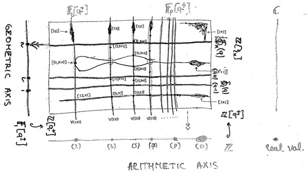
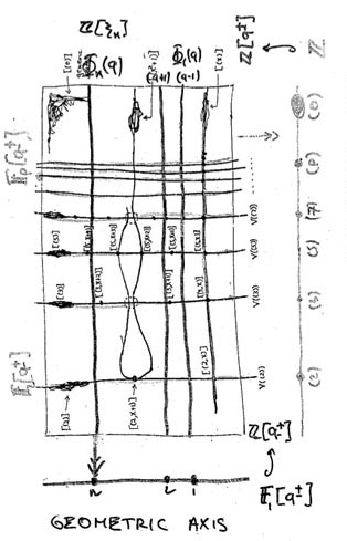
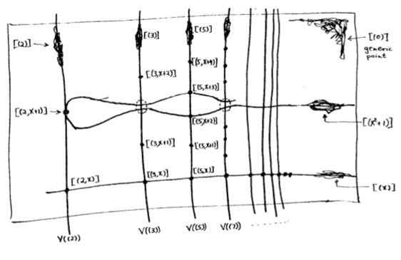
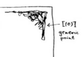
The doodle in the right upper corner depicts the ‘generic point’ of the scheme. That is, the geometric object corresponding to the prime ideal $~(0) $ (note that $\mathbb{Z}[x] $ is an integral domain). Because the zero ideal is contained in any other prime ideal, the algebraic/geometric mantra (“inclusions reverse when shifting between algebra and geometry”) asserts that the gemetric object corresponding to $~(0) $ should contain all other geometric objects of the arithmetic plane, so it is just the whole plane! Clearly, it is rather senseless to depict this fact by coloring the whole plane black as then we wouldn’t be able to see the finer objects. Mumford’s solution to this is to draw a hairy ball, which in this case, is sufficiently thick to include fragments going in every possible direction. In general, one should read these doodles as saying that the geometric object represented by this doodle contains all other objects seen elsewhere in the picture if the hairy-ball-doodle includes stuff pointing in the direction of the smaller object. So, in the case of the object corresponding to $~(0) $, the doodle has pointers going everywhere, saying that the geometric object contains all other objects depicted.

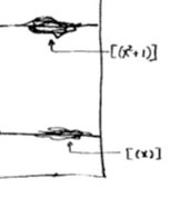
Let’s move over to the doodles in the lower right-hand corner. They represent the geometric object corresponding to principal prime ideals of the form $~(p(x)) $, where $p(x) $ in an irreducible polynomial over the integers, that is, a polynomial which we cannot write as the product of two smaller integral polynomials. The objects corresponding to such prime ideals should be thought of as ‘horizontal’ curves in the plane.

The doodles depicted correspond to the prime ideal $~(x) $, containing all polynomials divisible by $x $ so when we divide it out we get, as expected, a domain $\mathbb{Z}[x]/(x) \simeq \mathbb{Z} $, and the one corresponding to the ideal $~(x^2+1) $, containing all polynomials divisible by $x^2+1 $, which can be proved to be a prime ideals of $\mathbb{Z}[x] $ by observing that after factoring out we get $\mathbb{Z}[x]/(x^2+1) \simeq \mathbb{Z}[i] $, the domain of all Gaussian integers $\mathbb{Z}[i] $. The corresponding doodles (the ‘generic points’ of the curvy-objects) have a predominant horizontal component as they have the express the fact that they depict horizontal curves in the plane. It is no coincidence that the doodle of $~(x^2+1) $ is somewhat bulkier than the one of $~(x) $ as the later one must only depict the fact that all points lying on the straight line to its left belong to it, whereas the former one must claim inclusion of all points lying on the ‘quadric’ it determines.

Apart from these ‘horizontal’ curves, there are also ‘vertical’ lines corresponding to the principal prime ideals $~(p) $, containing the polynomials, all of which coefficients are divisible by the prime number $p $. These are indeed prime ideals of $\mathbb{Z}[x] $, because their quotients are
$\mathbb{Z}[x]/(p) \simeq (\mathbb{Z}/p\mathbb{Z})[x] $ are domains, being the ring of polynomials over the finite field $\mathbb{Z}/p\mathbb{Z} = \mathbb{F}_p $. The doodles corresponding to these prime ideals have a predominant vertical component (depicting the ‘vertical’ lines) and have a uniform thickness for all prime numbers $p $ as each of them only has to claim ownership of the points lying on the vertical line under them.

Right! So far we managed to depict the zero prime ideal (the whole plane) and the principal prime ideals of $\mathbb{Z}[x] $ (the horizontal curves and the vertical lines). Remains to depict the maximal ideals. These are all known to be of the form
$\mathfrak{m} = (p,f(x)) $
where $p $ is a prime number and $f(x) $ is an irreducible integral polynomial, which remains irreducible when reduced modulo $p $ (that is, if we reduce all coefficients of the integral polynomial $f(x) $ modulo $p $ we obtain an irreducible polynomial in $~\mathbb{F}_p[x] $). By the algebra/geometry mantra mentioned before, the geometric object corresponding to such a maximal ideal can be seen as the ‘intersection’ of an horizontal curve (the object corresponding to the principal prime ideal $~(f(x)) $) and a vertical line (corresponding to the prime ideal $~(p) $). Because maximal ideals do not contain any other prime ideals, there is no reason to have a doodle associated to $\mathfrak{m} $ and we can just depict it by a “point” in the plane, more precisely the intersection-point of the horizontal curve with the vertical line determined by $\mathfrak{m}=(p,f(x)) $. Still, Mumford’s treasure map doesn’t treat all “points” equally. For example, the point corresponding to the maximal ideal $\mathfrak{m}_1 = (3,x+2) $ is depicted by a solid dot $\mathbf{.} $, whereas the point corresponding to the maximal ideal $\mathfrak{m}_2 = (3,x^2+1) $ is represented by a fatter point $\circ $. The distinction between the two ‘points’ becomes evident when we look at the corresponding quotients (which we know have to be fields). We have

$\mathbb{Z}[x]/\mathfrak{m}_1 = \mathbb{Z}[x]/(3,x+2)=(\mathbb{Z}/3\mathbb{Z})[x]/(x+2) = \mathbb{Z}/3\mathbb{Z} = \mathbb{F}_3 $ whereas $\mathbb{Z}[x]/\mathfrak{m}_2 = \mathbb{Z}[x]/(3,x^2+1) = \mathbb{Z}/3\mathbb{Z}[x]/(x^2+1) = \mathbb{F}_3[x]/(x^2+1) = \mathbb{F}_{3^2} $

because the polynomial $x^2+1 $ remains irreducible over $\mathbb{F}_3 $, the quotient $\mathbb{F}_3[x]/(x^2+1) $ is no longer the prime-field $\mathbb{F}_3 $ but a quadratic field extension of it, that is, the finite field consisting of 9 elements $\mathbb{F}_{3^2} $. That is, we represent the ‘points’ lying on the vertical line corresponding to the principal prime ideal $~(p) $ by a solid dot . when their quotient (aka residue field is the prime field $~\mathbb{F}_p $, by a bigger point $\circ $ when its residue field is the finite field $~\mathbb{F}_{p^2} $, by an even fatter point $\bigcirc $ when its residue field is $~\mathbb{F}_{p^3} $ and so on, and on. The larger the residue field, the ‘fatter’ the corresponding point.

In fact, the ‘fat-point’ signs in Mumford’s treasure map are an attempt to depict the fact that an affine scheme contains a lot more information than just the set of all prime ideals. In fact, an affine scheme determines (and is determined by) a “functor of points”. That is, to every field (or even every commutative ring) the affine scheme assigns the set of its ‘points’ defined over that field (or ring). For example, the $~\mathbb{F}_p $-points of $\mathbf{spec}(\mathbb{Z}[x]) $ are the solid . points on the vertical line $~(p) $, the $~\mathbb{F}_{p^2} $-points of $\mathbf{spec}(\mathbb{Z}[x]) $ are the solid . points and the slightly bigger $\circ $ points on that vertical line, and so on.

This concludes our first attempt to decypher Mumford’s drawing, but if we delve a bit deeper, we are bound to find even more treasures… (to be continued).

Comments closed