Skip to content →

Tag: geometry

The Scottish solids hoax

A truly good math-story gets spread rather than scrutinized. And a good story it was : more than a millenium before Plato, the Neolithic Scottish Math Society classified the five regular solids : tetrahedron, cube, octahedron, dodecahedron and icosahedron. And, we had solid evidence to support this claim : the NSMS mass-produced stone replicas of their finds and about 400 of them were excavated, most of them in Aberdeenshire.

Six years ago, Michael Atiyah and Paul Sutcliffe arXived their paper Polyhedra in physics, chemistry and geometry, in which they wrote :

Although they are termed Platonic solids there is
convincing evidence that they were known to the Neolithic people of Scotland at least a
thousand years before Plato, as demonstrated by the stone models pictured in ๏ฌg. 1 which
date from this period and are kept in the Ashmolean Museum in Oxford.

Fig. 1 is the picture below, which has been copied in numerous blog-posts (including my own scottish solids-post) and virtually every talk on regular polyhedra.


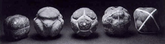
From left to right, stone-ball models of the cube, tetrahedron, dodecahedron, icosahedron and octahedron, in which ‘knobs’ correspond to ‘faces’ of the regular polyhedron, as best seen in the central dodecahedral ball.

But then … where’s the icosahedron? The fourth ball sure looks like one but only because someone added ribbons, connecting the centers of the different knobs. If this ribbon-figure is an icosahedron, the ball itself should be another dodecahedron and the ribbons illustrate the fact that icosa- and dodeca-hedron are dual polyhedra. Similarly for the last ball, if the ribbon-figure is an octahedron, the ball itself should be another cube, having exactly 6 knobs.
Who did adorn these artifacts with ribbons, thereby multiplying the number of ‘found’ regular solids by two (the tetrahedron is self-dual)?

The picture appears on page 98 of the book Sacred Geometry (first published in 1979) by Robert Lawlor. He attributes the NSMS-idea to the book Time Stands Still: New Light on Megalithic Science (also published in 1979) by Keith Critchlow. Lawlor writes

The five regular polyhedra or
Platonic solids were known and worked with
well before Plato’s time. Keith Critchlow in
his book Time Stands Still presents convincing
evidence that they were known to the Neolithic peoples of Britain at least 1000 years
before Plato. This is founded on the existence
of a number of sphericalfstones kept in the
Ashmolean Museum at Oxford. Of a size one
can carry in the hand, these stones were carved
into the precise geometric spherical versions of
the cube, tetrahedron, octahedron, icosahedron
and dodecahedron, as well as some additional
compound and semi-regular solids, such as the
cube-octahedron and the icosidodecahedron.
Critchlow says, ‘What we have are objects
clearly indicative of a degree of mathematical
ability so far denied to Neolithic man by any
archaeologist or mathematical historian’. He
speculates on the possible relationship of these
objects to the building of the great astronomical stone circles of the same epoch in Britain:
‘The study of the heavens is, after all, a
spherical activity, needing an understanding of
spherical coordinates. If the Neolithic inhabitants of Scotland had constructed Maes Howe
before the pyramids were built by the ancient
Egyptians, why could they not be studying the
laws of three-dimensional coordinates? Is it not
more than a coincidence that Plato as well as
Ptolemy, Kepler and Al-Kindi attributed
cosmic significance to these figures?’

As Lawlor and Critchlow lean towards mysticism, their claims should not be taken for granted. So, let’s have a look at these famous stones kept in the Ashmolean Museum. The Ashmolean has a page dedicated to their Stone Balls, including the following picture (the Critchlow/Lawlor picture below, for comparison)


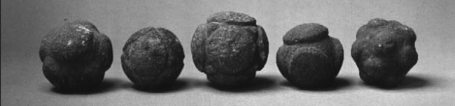
The Ashmolean stone balls are from left to right the artifacts with catalogue numbers :

  • Stone ball with 7 knobs from Marnoch, Banff (AN1927.2728)
  • Stone ball with 6 knobs and isosceles triangles between, from Fyvie, Aberdeenshire (AN1927.2731)
  • Stone ball with 6 knobs and isosceles triangles between, from near Aberdeen (AN1927.2730)
  • Stone ball with 4 knobs from Auchterless, Aberdeenshire (AN1927.2729)
  • Stone ball with 14 knobs from Aberdeen (AN1927.2727)

Ashmolean’s AN 1927.2729 may very well be the tetrahedron and AN 1927.2727 may be used to forge the ‘icosahedron’ (though it has 14 rather than 12 knobs), but the other stones sure look different. In particular, none of the Ashmolean stones has exactly 12 knobs in order to be a dodecahedron.

Perhaps the Ashmolean has a larger collection of Scottish balls and today’s selection is different from the one in 1979? Well, if you have the patience to check all 9 pages of the Scottish Ball Catalogue by Dorothy Marshall (the reference-text when it comes to these balls) you will see that the Ashmolean has exactly those 5 balls and no others!

The sad lesson to be learned is : whether the Critchlow/Lawlor balls are falsifications or fabrications, they most certainly are NOT the Ashmolean stone balls as they claim!

Clearly this does not mean that no neolithic scott could have discovered some regular polyhedra by accident. They made an enormous amount of these stone balls, with knobs ranging from 3 up to no less than 135! All I claim is that this ball-carving thing was more an artistic endeavor, rather than a mathematical one.

There are a number of musea having a much larger collection of these stone balls. The Hunterian Museum has a collection of 29 and some nice online pages on them, including 3D animation. But then again, none of their balls can be a dodecahedron or icosahedron (according to the stone-ball-catalogue).

In fact, more than half of the 400+ preserved artifacts have 6 knobs. The catalogue tells that there are only 8 possible candidates for a Scottish dodecahedron (below their catalogue numbers, indicating for the knowledgeable which museum owns them and where they were found)

  • NMA AS 103 : Aberdeenshire
  • AS 109 : Aberdeenshire
  • AS 116 : Aberdeenshire (prob)
  • AUM 159/9 : Lambhill Farm, Fyvie, Aberdeenshire
  • Dundee : Dyce, Aberdeenshire
  • GAGM 55.96 : Aberdeenshire
  • Montrose = Cast NMA AS 26 : Freelands, Glasterlaw, Angus
  • Peterhead : Aberdeenshire

The case for a Scottish icosahedron looks even worse. Only two balls have exactly 20 knobs

  • NMA AS 110 : Aberdeenshire
  • GAGM 92 106.1. : Countesswells, Aberdeenshire

Here NMA stands for the National Museum of Antiquities of Scotland in Edinburg (today, it is called ‘National Museums Scotland’) and
GAGM for the Glasgow Art Gallery and Museum. If you happen to be in either of these cities shortly, please have a look and let me know if one of them really is an icosahedron!

UPDATE (April 1st)

Victoria White, Curator of Archaeology at the
Kelvingrove Art Gallery and Museum, confirms that the Countesswells carved stone ball (1892.106.l) has indeed 20 knobs. She gave this additional information :

The artefact came to Glasgow Museums in the late nineteenth century as part of the John Rae collection. John Rae was an avid collector of prehistoric antiquities from the Aberdeenshire area of Scotland. Unfortunately, the ball was not accompanied with any additional information regarding its archaeological context when it was donated to Glasgow Museums. The carved stone ball is currently on display in the ‘Raiders of the Lost Art’ exhibition.

Dr. Alison Sheridan, Head of Early Prehistory, Archaeology Department, National Museums Scotland makes the valid point that new balls have been discovered after the publication of the catalogue, but adds :

Although several balls have turned up since Dorothy Marshall wrote her synthesis, none has 20 knobs, so you can rely on Dorothyโ€™s list.

She has strong reservations against a mathematical interpretation of the balls :

Please also note that the mathematical interpretation of these Late Neolithic objects fails to take into account their archaeological background, and fails to explain why so many do not have the requisite number of knobs! Itโ€™s a classic case of people sticking on an interpretation in a state of ignorance. A great shame when so much is known about Late Neolithic archaeology.

2 Comments

Geometry of the Okubo algebra

Last week, Melanie Raczek gave a talk entitled ‘Cubic forms and Okubo product’ in our Artseminar, based on her paper On ternary cubic forms that determine central simple algebras of degree 3.

I had never heard of this strange non-associative product on 8-dimensional space, but I guess it is an instance of synchronicity that now the Okubo algebra seems to pop-up everywhere.

Yesterday, there was the post the Okubo algebra by John Baez at the n-cafe, telling that Susumu Okubo discovered his algebra while investigating quarks.

I don’t know a thing about the physics, but over the last days I’ve been trying to understand some of the miraculous geometry associated to the Okubo algebra. So, let’s start out by defining the ‘algebra’.

Consider the associative algebra of all 3×3 complex matrices $M_3(\mathbb{C}) $ with the usual matrix-multiplication. In this algebra there is the 8-dimensional subspace of trace zero matrices, usually called the Lie algebra $\mathfrak{sl}_3 $. However, we will not use the Lie-bracket, only matrix-multiplication. Typical elements of $\mathfrak{sl}_3 $ will be written as $X,Y,Z,… $ and their entries will be denoted as

$X = \begin{bmatrix} x_0 & x_1 & x_2 \\ x_3 & x_4 & x_5 \\ x_6 & x_7 & -x_0-x_4 \end{bmatrix} $

For any two elements $X,Y \in \mathfrak{sl}_3 $ one defines their Okubo-product to be the 3×3 matrix

$X \ast Y = \frac{1}{1-\omega}(Y.X-\omega X.Y) – \frac{1}{3}Tr(X.Y) 1_3 $

where $\omega $ is a primitive 3-rd root of unity and $1_3 $ is the identity matrix. Written out in the entries of X and Y this operation looks horribly complicated

$X \ast Y = \frac{1}{1-\omega} \begin{bmatrix} p_{11} & p_{12} & p_{13} \\ p_{21} & p_{22} & p_{23} \\ p_{31} & p_{32} & -p_{11}-p_{22} \end{bmatrix} $

with

[tex]\begin{eqalign} \\ p_{11} &= (1-\omega)x_0y_0+x_3y_1+x_6y_2-\omega(x_1y_3+x_2y_6)-\frac{1}{3}T \\ p_{12} &= x_1y_0+x_4y_1+x_7y_2-\omega(x_0y_1+x_1y_4+x_2y_7) \\ p_{13} &= x_2y_0+x_5y_1-x_0y_2-x_4y_2-\omega(x_0y_2+x_1y_5-x_2y_0-x_2y_4) \\
p_{21} &= x_0y_3+x_3y_4+x_6y_5 – \omega(x_3y_0+x_4y_3+x_5y_6) \\
p_{22} &= (1-\omega)x_4y_4+x_1y_3+x_7y_5 – \omega(x_3y_1+x_5y_7) – \frac{1}{3}T \\
p_{23} &= x_2y_3+x_5y_4-x_0y_5-x_4y_5-\omega(x_3y_2+x_4y_5-x_5y_0-x_5y_4) \\
p_{31} &= x_0y_6+x_3y_7-x_6y_0-x_6y_4-\omega(x_6y_0+x_7y_3-x_0y_6-x_4y_6) \\
p_{32} &= x_1y_6+x_4y_7-x_7y_0-x_7y_4 – \omega(x_6y_1+x_7y_4-x_0y_7-x_4y_7) \\
T &= 2x_0y_0+2x_4y_4+x_1y_3+x_2y_6+x_3y_1+x_5y_7+x_6y_2+x_7y_5+x_0y_4+x_4y_0
\end{eqalign}[/tex]

The crucial remark to make is that $X \ast Y $ is again a trace zero matrix. That is, we have defined a new operation on $\mathfrak{sl}_3 $.

$\mathfrak{sl}_3 \times \mathfrak{sl}_3 \rightarrow \mathfrak{sl}_3~\qquad~\qquad~(X,Y) \mapsto X \ast Y $

This Okubo-product is neither a Lie-bracket, nor an associative multiplication. In fact, it is a lot ‘less associative’ than that other 8-dimensional algebra, the octonions. The only noteworthy identity it has is that $X \ast (Y \ast X) = (X \ast Y) \ast X $. So, why should we be interested in this horrible algebra?

Well, let us consider the subset of $\mathfrak{sl}_3 $ consisting of those matrices X satusfying $Tr(X^2)=0 $. That is, with the above notation, all matrices X such that

$x_0^2+x_4^2+x_1x_3+x_2x_6+x_5x_7=0 $

In the 8-dimensional affine space $\mathfrak{sl}_3 $ these matrices form a singular quadric with top the zero-matrix. So, it is better to go projective. That is, any non-zero matrix $X \in \mathfrak{sl}_3 $ determines a point in 7-dimensional projective space $\mathbb{P}^7 $ with homogeneous coordinates

$\overline{X} = [x_0:x_1:x_2:x_3:x_4:x_5:x_6:x_7] \in \mathbb{P}^7 $

and the points $\overline{X} $ corresponding to solutions of $Tr(X^2)=0 $ form a smooth 6-dimensional quadric $Q \subset \mathbb{P}^7 $ with homogeneous equation

$Q = \mathbb{V}(x_0^2+x_4^2+x_1x_3+x_2x_6+x_5x_7) $

6-dimensional quadrics may be quite hard to visualize, so it may help to recall the classic situation of lines on a 2-dimensional quadric (animated gif taken from surfex).

A 2-dimensional quadric contains two families of lines, often called the ‘blue lines’ and the ‘red lines’, each of these lines isomorphic to $\mathbb{P}^1 $. The rules-of-intersection of these are :

  • different red lines are disjoint as are different blue lines
  • any red and any blue line intersect in exactly one point
  • every point of the quadric lies on exactly one red and one blue line

The lines in either family are in one-to-one correspondence with the points on the projective line. We therefore say that there is a $\mathbb{P}^1 $-family of red lines and a $\mathbb{P}^1 $-family of blue lines on a 2-dimensional quadric.

A 6-dimensional quadric $Q \subset \mathbb{P}^7 $ contains two families of ‘3-planes’. That is, there is a family of red $\mathbb{P}^3 $’s contained in Q and a family of blue $\mathbb{P}^3 $’s. Can we determine these red and blue 3-planes explicitly?

Yes we can, using the Okubo algebra-product on $\mathfrak{sl}_3 $. Take $X \in \mathfrak{sl}_3 $ defining the point $\overline{X} \in Q $ (that is, $Tr(X^2)=0 $). then all 3×3 matrices one obtains by taking the Okubo-product with left X-factor form a 4-dimensional linear subspace in $\mathfrak{sl}_3 $

$L_X = { X \ast Y~|~Y \in \mathfrak{sl}_3 } \simeq \mathbb{C}^4 \subset \mathfrak{sl}_3 $

so its non-zero matrices determine a 3-plane in $\mathbb{P}^7 $ (consisting of all points with homogeneous coordinates $[p_{11}:p_{12}:p_{13}:p_{21}:p_{22}:p_{23}:p_{31}:p_{32}] $, using the above formulas) which actually lies entirely in the quadric Q. These are precisely the bLue 3-planes in Q. That is, the family of all bLue 3-planes consists precisely of the 3-planes

$\mathbb{P}(L_X) $ with $X \in \mathfrak{sl}_3 $ satisfying $Tr(X^2)=0 $

Phrased differently, any point $\overline{X} \in Q $ determines a blue 3-plane $\mathbb{P}(L_X) $.

Similarly, any point $\overline{X} \in Q $ determines a Red 3-plane by taking Okubo-products with Right X-factor, that is, $\mathbb{P}(R_X) $ is a 3-plane for Q where

$R_X = { Y \ast X~|~Y \in \mathfrak{sl}_3 } \simeq \mathbb{C}^4 \subset \mathfrak{sl}_3 $

and all Red 3-planes for Q are of this form. But, this is not all… these correspondences are unique! That is, any point on the quadric defines a unique red and a unique blue 3-plane, or, phrased differently, there is a Q-family of red 3-planes and a Q-family of blue 3-planes in Q. This is a consequence of triality.

To see this, note that the automorphism group of a 6-dimensional smooth quadric is the rotation group $SO_8(\mathbb{C}) $ and this group has Dynkin diagram $D_4 $, the most symmetrical of them all!

In general, every node in a Dynkin diagram has an interesting projective variety associated to it, a so called homogeneous space. I’ll just mention what these spaces are corresponding to the 4 nodes of $D_4 $. Full details can be found in chapter 23 of Fulton and Harris’ Representation theory, a first course.

The left-most node corresponds to the orthogonal Grassmannian of isotropic 1-planes in $\mathbb{C}^8 $ which is just a fancy way of viewing our quadric Q. The two right-most nodes correspond to the two connected components of the Grassmannians of isotropic 4-planes in $\mathbb{C}^8 $, which are our red resp. blue families of 3-planes on the quadric. Now, as the corresponding dotted Dynkin diagrams are isomorphic


there corresponding homogeneous spaces are also isomorphic. Thus indeed, there is a one-to-one correspondence between points of the quadric Q and red 3-planes on Q (and similarly with blue 3-planes on Q).

Okay, so the Okubo-product allows us to associate to a point on the 6-dimensional quadric Q a unique red 3-plane and a unique blue 3-plane (much as any point on a 2-dimensional quadric determines a unique red and blue line). Do these families of red and blue 3-planes also satisfy ‘rules-of-intersection’?

Yes they do and, once again, the Okubo-product clarifies them. Here they are :

  • two different red 3-planes intersect in a unique line (as do different blue 3-planes)
  • the bLue 3-plane $\mathbb{P}(L_X) $ intersects the Red 3-plane $\mathbb{P}(R_Y) $ in a unique point if and only if the Okubo-product $X \ast Y \not= 0 $
  • the bLue 3-plane $\mathbb{P}(L_X) $ intersects the Red 3-plane $\mathbb{P}(R_Y) $ in a unique 2-plane if and only if the Okubo-product $X \ast Y = 0 $

That is, Right and Left Okubo-products determine the Red and bLue families of 3-planes on the 6-dimensional quadric as well as their intersections!

Comments closed

Connes & Consani go categorical

Today, Alain Connes and Caterina Consani arXived their new paper Schemes over $ \mathbb{F}_1$ and zeta functions. It is a follow-up to their paper On the notion of geometry over $ \mathbb{F}_1$, which I’ve tried to explain in a series of posts starting here.

As Javier noted already last week when they updated their first paper, the main point of the first 25 pages of the new paper is to repace abelian groups by abelian monoids in the definition, making it more in tune with other approaches, most notably that of Anton Deitmar. The novelty, if you want, is that they package the two functors $\mathbf{rings} \rightarrow \mathbf{sets} $ and $\mathbf{ab-monoid} \rightarrow \mathbf{sets} $ into one functor $\mathbf{ring-monoid} \rightarrow \mathbf{sets} $ by using the ‘glued category’ $\mathbf{ring-monoid} $ (an idea they attribute to Pierre Cartier).

In general, if you have two categories $\mathbf{cat} $ and $\mathbf{cat’} $ and a pair of adjoint functors between them, then one can form the glued-category $\mathbf{cat-cat’} $ by taking as its collection of objects the disjoint union of the objects of the two categories and by defining the hom-sets between two objects the hom-sets in either category (if both objects belong to the same category) or use the adjoint functors to define the new hom-set when they do not (the very definition of adjoint functors makes that this doesn’t depend on the choice).

Here, one uses the functor $\mathbf{ab-monoid} \rightarrow \mathbf{rings} $ assigning to a monoid $M $ its integral monoid-algebra $\mathbb{Z}[M] $, having as its adjoint the functor $\mathbf{rings} \rightarrow \mathbf{ab-monoid} $ forgetting the additive structure of the commutative ring.

In the second part of the paper, they first prove some nice results on zeta-functions of Noetherian $\mathbb{F}_1 $-schemes and extend them, somewhat surprisingly, to settings which do not (yet) fit into the $\mathbb{F}_1 $-framework, namely elliptic curves and the hypothetical $\mathbb{F}_1 $-curve $\overline{\mathbf{spec}(\mathbb{Z})} $.

Comments closed