Learners’ logic

In the Learners and Poly-post we’ve seen that learners from $A$ to $B$ correspond to set-valued representations of a directed graph $G$ and therefore form a presheaf topos.

Any topos comes with its Mitchell-Benabou language, allowing us to speak of formulas, propositions and their truth values. Two objects play a special role in this: the terminal object $\mathbf{1}$, and the subobject classifier $\mathbf{\Omega }$. It is a fun exercise to determine these special learners.

$T$ is the free rooted tree with branches sprouting from every node $n\in T_0$ for each element in $A\times B$. $C$ will be our set of colours, one for each element of $Maps(A,B)\times Maps(A\times B,A)$.

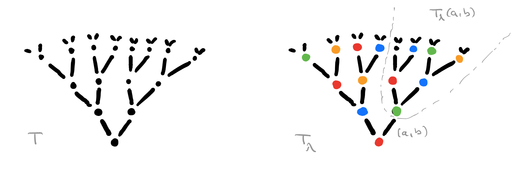
For every map $\lambda :T_0\to C$ we get a coloured rooted tree $T_{\lambda }$, and for each branch $(a,b)$ from the root we get another rooted sub-tree $T_{\lambda }(a,b)$ which is again of the form $T_{\mu }$ for a certain map $\mu :T_0\to C$.

The directed graph $G$ has a vertex $v_{\lambda }\in V$ for each coloured rooted tree $T_{\lambda }$ and a directed edge $v_{\lambda }\to v_{\mu }$ if $T_{\mu }$ is the isomorphism class of coloured rooted trees of the subtree $T_{\lambda }(a,b)$ for some $(a,b)\in A\times B$.

There are exactly $\mathrm{\#}A\times B$ directed edges leaving every vertex in $G$, but there may be (many) more incoming edges. We can colour each vertex $v_{\lambda }$ with the colour of the root of $T_{\lambda }$.

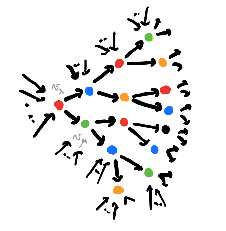
The coloured directed graph $G$ depicts the learning process in a neural network, being trained to find a suitable map $A\to B$. The colour of a vertex $v_{\lambda }$ gives a map $f\in Maps(A,B)$ (and a request function). If the network now gives as output $b\in B$ for a given input $a\in A$, we can move on to the end-vertex $v_{\mu }$ of the directed edge labeled $(a,b)$ out of $v_{\lambda }$. The colour of $v_{\mu }$ gives us a new (hopefully improved) map $f_{new}\in Maps(A,B)$ (and a new request function). A new training data $(a^{\prime },b^{\prime })$ brings us to a new vertex and map, and so on.

Clearly, some parts of $G$ are more efficient to find the desired map than others, and the aim of the game is to distinguish efficient from inefficient learners. A first hint that Grothendieck topologies and their corresponding sheafifications will turn out to be important.

We’ve seen that a learner, that is a morphism $P{y}^P\to C{y}^{A\times B}$ in $\mathbf{Poly}$, assigns a set $P_{\lambda }$ to every vertex $v_{\lambda }$ (this set may be empty) and a map $P_{\lambda }\to P_{\mu }$ to every directed edge $v_{\lambda }\to v_{\mu }$ in $G$.

The terminal object $\mathbf{1}$ in this setting assigns to each vertex a singleton $\{\ast \}$, and the obvious maps for each directed edge. In $\mathbf{Poly}$-speak, the terminal object is the morphism
$$\mathbf{1}:V{y}^V\to C{y}^{A\times B}$$
which sends each vertex $v_{\lambda }\in V$ to its colour $c\in C$, and where the backtrack map ${\phi }_{v_{\lambda }}^{\mathrm{\#}}[c]$ maps $(a,b)$ to $v_{\mu }$ if this is the end-vertex of the edge labelled $(a,b)$ out of $v_{\lambda }$. That is, $\mathbf{1}$ contains all information about the coloured directed graph $G$.

The subobject classifier $\mathbf{\Omega }$ assigns to each vertex $v_{\lambda }$ the set $\mathbf{\Omega }(v_{\lambda })$ of all subsets $S$ of directed paths in $G$, starting at $v_{\lambda }$, such that if $p\in S$ then also all prolongated paths belong to $S$. Note that the emptyset $\mathrm{\varnothing }$ satisfies this requirement, so is an element of this vertex set. Another special element in $\mathbf{\Omega }(v_{\lambda })$ is the set ${\mathbf{1}}_{\lambda }$ of all oriented paths starting at $v_{\lambda }$.

$\mathbf{\Omega }(v_{\lambda })$ is an Heyting algebra with $1={\mathbf{1}}_{\lambda }$, $0=\mathrm{\varnothing }$, partially ordered via inclusion, and logical operations $\wedge$ (intersection), $\vee$ (union), $\mathrm{\neg }$ (with $\mathrm{\neg }S$ the largest $S^{\prime }\in \mathbf{\Omega }(v_{\lambda })$ disjoint from $S$) and $\Rightarrow$ defined by $S\Rightarrow S^{\prime }$ is the union of all $S”\in \mathbf{\Omega }(v_{\lambda })$ such that $S”\cap S\subseteq S^{\prime }$.

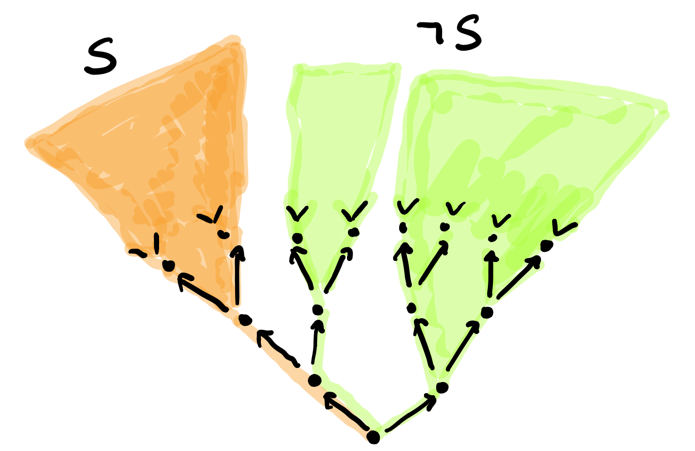
$S\wedge \mathrm{\neg }S$ is not always equal to $1$. Here, the union misses the left edge from the root. So, we will not be able to prove things by contradiction.

If $v_{\lambda }\to v_{\mu }$ is the directed edge labeled $(a,b)$, then the corresponding map $\mathbf{\Omega }(v_{\lambda })\to \mathbf{\Omega }(v_{\mu })$ takes an $S\in \mathbf{\Omega }(v_{\lambda })$, drops all paths which do not pass through $v_{\mu }$ and removes from those who do the initial edge $(a,b)$. If no paths in $S$ pass through $v_{\mu }$ then $S$ is mapped to $\mathrm{\varnothing }\in \mathbf{\Omega }(v_{\mu })$.

If $\mathrm{\Omega }=\underset{\lambda }{⨆}\mathbf{\Omega }(v_{\lambda })$ then the subobject classifier is the morphism in $\mathbf{Poly}$
$$\mathbf{\Omega }:\mathrm{\Omega }{y}^{\mathrm{\Omega }}\to C{y}^{A\times B}$$
sending a path starting in $v_{\lambda }$ to the colour of $v_{\lambda }$ and the backtrack map of $(a,b)$ the image of the path under the map $\mathbf{\Omega }(v_{\lambda })\to \mathbf{\Omega }(v_{\mu })$.

Ok, let’s define the Learner’s Mitchell-Benabou language.

We’ll view a learner $P{y}^P\to C{y}^{A\times B}$ as a set-valued representation $P$ of the directed graph $G$ with vertex set $P_{\lambda }$ placed at vertex $v_{\lambda }$.

A formula $\varphi (p)$ of the language with a free variable $p$ is a morphism (of representations of $G$) from a learner $P$ to the subobject classifier
$$\varphi :P\to \mathbf{\Omega }$$
Such a morphism determines a sub-representation of $P$ which we can denote $\{p|\varphi (p)\}$ with vertex sets
$$\{p|\varphi (p){\}}_{\lambda }=\{p\in P_{\lambda }|\varphi (v_{\lambda })(p)={\mathbf{1}}_{\lambda }\}$$

On formulas we can apply logical connectives to get more formulas. For example, the formula $\varphi (p)\Rightarrow \psi (q)$ is the composition
$$P\times Q{\to }^{\varphi \times \psi }\mathbf{\Omega }\times \mathbf{\Omega }{\to }^{\Rightarrow }\mathbf{\Omega }$$

By quantifying all free variables we get a formula without free variables, and those correspond to morphisms $\mathbf{1}\to \mathbf{\Omega }$, that is, to sub-representations of the terminal object $\mathbf{1}$.

For example, if $\varphi (p)$ is the formula with free variable $p$ corresponding to the morphism $\varphi :P\to \mathbf{\Omega }$, then we have
$$\mathrm{\forall }p:\varphi (p)=\{v_{\lambda }\in V|\{p|\varphi (p){\}}_{\lambda }=P_{\lambda }\}$$
and
$$\mathrm{\exists }p:\varphi (p)=\{v_{\lambda }\in V|\{p|\varphi (p){\}}_{\lambda }\ne \mathrm{\varnothing }\}$$

Sub-representations of $\mathbf{1}$ again form a Heyting-algebra in the obvious way, so we can assign a “truth-value” to a formula without free variables as that sub-object of $\mathbf{1}$.

There’s a lot more to say, so perhaps this will be continued.