representations – Page 4 – neverendingbooks

A standard Grassmannian $Gr(m,V)$ is the manifold having as its points all possible $m$-dimensional subspaces of a given vectorspace $V$. As an example, $Gr(1,V)$ is the set of lines through the origin in $V$ and therefore is the projective space $\mathbb{P}(V)$. Grassmannians are among the nicest projective varieties, they are smooth and allow a cell decomposition.

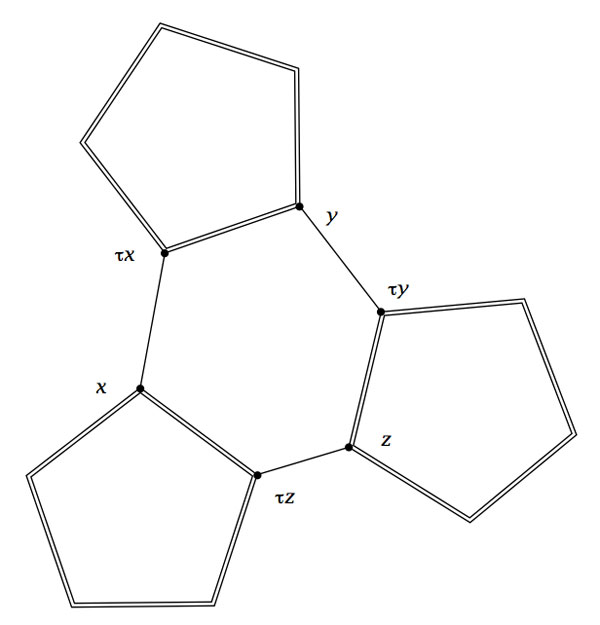
A quiver $Q$ is just an oriented graph. Here’s an example

A representation $V$ of a quiver assigns a vector-space to each vertex and a linear map between these vertex-spaces to every arrow. As an example, a representation $V$ of the quiver $Q$ consists of a triple of vector-spaces $(V_1,V_2,V_3)$ together with linear maps $f_a~:~V_2 \rightarrow V_1$ and $f_b,f_c~:~V_2 \rightarrow V_3$.

A sub-representation $W \subset V$ consists of subspaces of the vertex-spaces of $V$ and linear maps between them compatible with the maps of $V$. The dimension-vector of $W$ is the vector with components the dimensions of the vertex-spaces of $W$.

This means in the example that we require $f_a(W_2) \subset W_1$ and $f_b(W_2)$ and $f_c(W_2)$ to be subspaces of $W_3$. If the dimension of $W_i$ is $m_i$ then $m=(m_1,m_2,m_3)$ is the dimension vector of $W$.

The quiver-analogon of the Grassmannian $Gr(m,V)$ is the Quiver Grassmannian $QGr(m,V)$ where $V$ is a quiver-representation and $QGr(m,V)$ is the collection of all possible sub-representations $W \subset V$ with fixed dimension-vector $m$. One might expect these quiver Grassmannians to be rather nice projective varieties.

However, last week Markus Reineke posted a 2-page note on the arXiv proving that every projective variety is a quiver Grassmannian.

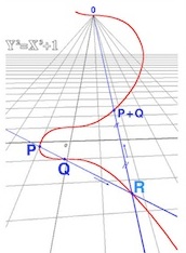
Let’s illustrate the argument by finding a quiver Grassmannian $QGr(m,V)$ isomorphic to the elliptic curve in $\mathbb{P}^2$ with homogeneous equation $Y^2Z=X^3+Z^3$.

Consider the Veronese embedding $\mathbb{P}^2 \rightarrow \mathbb{P}^9$ obtained by sending a point $(x:y:z)$ to the point

\[ (x^3:x^2y:x^2z:xy^2:xyz:xz^2:y^3:y^2z:yz^2:z^3) \]

The upshot being that the elliptic curve is now realized as the intersection of the image of $\mathbb{P}^2$ with the hyper-plane $\mathbb{V}(X_0-X_7+X_9)$ in the standard projective coordinates $(x_0:x_1:\cdots:x_9)$ for $\mathbb{P}^9$.

To describe the equations of the image of $\mathbb{P}^2$ in $\mathbb{P}^9$ consider the $6 \times 3$ matrix with the rows corresponding to $(x^2,xy,xz,y^2,yz,z^2)$ and the columns to $(x,y,z)$ and the entries being the multiplications, that is

$$\begin{bmatrix} x^3 & x^2y & x^2z \\ x^2y & xy^2 & xyz \\ x^2z & xyz & xz^2 \\ xy^2 & y^3 & y^2z \\ xyz & y^2z & yz^2 \\ xz^2 & yz^2 & z^3 \end{bmatrix} = \begin{bmatrix} x_0 & x_1 & x_2 \\ x_1 & x_3 & x_4 \\ x_2 & x_4 & x_5 \\ x_3 & x_6 & x_7 \\ x_4 & x_7 & x_8 \\ x_5 & x_8 & x_9 \end{bmatrix}$$

But then, a point $(x_0:x_1: \cdots : x_9)$ belongs to the image of $\mathbb{P}^2$ if (and only if) the matrix on the right-hand side has rank $1$ (that is, all its $2 \times 2$ minors vanish). Next, consider the quiver

and consider the representation $V=(V_1,V_2,V_3)$ with vertex-spaces $V_1=\mathbb{C}$, $V_2 = \mathbb{C}^{10}$ and $V_2 = \mathbb{C}^6$. The linear maps $x,y$ and $z$ correspond to the columns of the matrix above, that is

$$(x_0,x_1,x_2,x_3,x_4,x_5,x_6,x_7,x_8,x_9) \begin{cases} \rightarrow^x~(x_0,x_1,x_2,x_3,x_4,x_5) \\ \rightarrow^y~(x_1,x_3,x_4,x_6,x_7,x_8) \\ \rightarrow^z~(x_2,x_4,x_5,x_7,x_8,x_9) \end{cases}$$

The linear map $h~:~\mathbb{C}^{10} \rightarrow \mathbb{C}$ encodes the equation of the hyper-plane, that is $h=x_0-x_7+x_9$.

Now consider the quiver Grassmannian $QGr(m,V)$ for the dimension vector $m=(0,1,1)$. A base-vector $p=(x_0,\cdots,x_9)$ of $W_2 = \mathbb{C}p$ of a subrepresentation $W=(0,W_2,W_3) \subset V$ must be such that $h(x)=0$, that is, $p$ determines a point of the hyper-plane.

Likewise the vectors $x(p),y(p)$ and $z(p)$ must all lie in the one-dimensional space $W_3 = \mathbb{C}$, that is, the right-hand side matrix above must have rank one and hence $p$ is a point in the image of $\mathbb{P}^2$ under the Veronese.

That is, $Gr(m,V)$ is isomorphic to the intersection of this image with the hyper-plane and hence is isomorphic to the elliptic curve.

The general case is similar as one can view any projective subvariety $X \rightarrow \mathbb{P}^n$ as isomorphic to the intersection of the image of a specific $d$-uple Veronese embedding $\mathbb{P}^n \rightarrow \mathbb{P}^N$ with a number of hyper-planes in $\mathbb{P}^N$.

ADDED For those desperate to read the original comments-section, here’s the link.

Comments closed

We saw that the icosahedron can be constructed from the alternating group $A_5 $ by considering the elements of a conjugacy class of order 5 elements as the vertices and edges between two vertices if their product is still in the conjugacy class.

This description is so nice that one would like to have a similar construction for the buckyball. But, the buckyball has 60 vertices, so they surely cannot correspond to the elements of a conjugacy class of $A_5 $. But, perhaps there is a larger group, somewhat naturally containing $A_5 $, having a conjugacy class of 60 elements?

This is precisely the statement contained in Galois’ last letter. He showed that 11 is the largest prime p such that the group $L_2(p)=PSL_2(\mathbb{F}_p) $ has a (transitive) permutation presentation on p elements. For, p=11 the group $L_2(11) $ is of order 660, so it permuting 11 elements means that this set must be of the form $X=L_2(11)/A $ with $A \subset L_2(11) $ a subgroup of 60 elements… and it turns out that $A \simeq A_5 $…

Actually there are TWO conjugacy classes of subgroups isomorphic to $A_5 $ in $L_2(11) $ and we have already seen one description of these using the biplane geometry (one class is the stabilizer subgroup of a ‘line’, the other the stabilizer subgroup of a point).

Here, we will give yet another description of these two classes of $A_5 $ in $L_2(11) $, showing among other things that the theory of dessins d’enfant predates Grothendieck by 100 years.

In the very same paper containing the first depiction of the Dedekind tessellation, Klein found that there should be a degree 11 cover $\mathbb{P}^1_{\mathbb{C}} \rightarrow \mathbb{P}^1_{\mathbb{C}} $ with monodromy group $L_2(11) $, ramified only in the three points ${ 0,1,\infty } $ such that there is just one point lying over $\infty $, seven over 1 of which four points where two sheets come together and finally 5 points lying over 0 of which three where three sheets come together. In 1879 he wanted to determine this cover explicitly in the paper “Ueber die Transformationen elfter Ordnung der elliptischen Funktionen” (Math. Annalen) by describing all Riemann surfaces with this ramification data and pick out those with the correct monodromy group.

He manages to do so by associating to all these covers their ‘dessins d’enfants’ (which he calls Linienzuges), that is the pre-image of the interval [0,1] in which he marks the preimages of 0 by a bullet and those of 1 by a +, such as in the innermost darker graph on the right above. He even has these two wonderful pictures explaining how the dessin determines how the 11 sheets fit together. (More examples of dessins and the correspondences of sheets were drawn in the 1878 paper.)

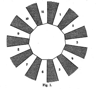
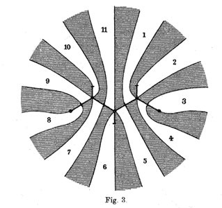
The ramification data translates to the following statements about the Linienzuge : (a) it must be a tree ($\infty $ has one preimage), (b) there are exactly 11 (half)edges (the degree of the cover),
(c) there are 7 +-vertices and 5 o-vertices (preimages of 0 and 1) and (d) there are 3 trivalent o-vertices and 4 bivalent +-vertices (the sheet-information).

Klein finds that there are exactly 10 such dessins and lists them in his Fig. 2 (left). Then, he claims that one the two dessins of type I give the correct monodromy group. Recall that the monodromy group is found by giving each of the half-edges a number from 1 to 11 and looking at the permutation $\tau $ of order two pairing the half-edges adjacent to a +-vertex and the order three permutation $\sigma $ listing the half-edges by cycling counter-clockwise around a o-vertex. The monodromy group is the group generated by these two elements.

Fpr example, if we label the type V-dessin by the numbers of the white regions bordering the half-edges (as in the picture Fig. 3 on the right above) we get
$\sigma = (7,10,9)(5,11,6)(1,4,2) $ and $\tau=(8,9)(7,11)(1,5)(3,4) $.

Nowadays, it is a matter of a few seconds to determine the monodromy group using GAP and we verify that this group is $A_{11} $.

Of course, Klein didn’t have GAP at his disposal, so he had to rule out all these cases by hand.

gap> g:=Group((7,10,9)(5,11,6)(1,4,2),(8,9)(7,11)(1,5)(3,4));
Group([ (1,4,2)(5,11,6)(7,10,9), (1,5)(3,4)(7,11)(8,9) ])
gap> Size(g);
19958400
gap> IsSimpleGroup(g);
true

Klein used the fact that $L_2(11) $ only has elements of orders 1,2,3,5,6 and 11. So, in each of the remaining cases he had to find an element of a different order. For example, in type V he verified that the element $\tau.(\sigma.\tau)^3 $ is equal to the permutation (1,8)(2,10,11,9,6,4,5)(3,7) and consequently is of order 14.

Perhaps Klein knew this but GAP tells us that the monodromy group of all the remaining 8 cases is isomorphic to the alternating group $A_{11} $ and in the two type I cases is indeed $L_2(11) $. Anyway, the two dessins of type I correspond to the two conjugacy classes of subgroups $A_5 $ in the group $L_2(11) $.

But, back to the buckyball! The upshot of all this is that we have the group $L_2(11) $ containing two classes of subgroups isomorphic to $A_5 $ and the larger group $L_2(11) $ does indeed have two conjugacy classes of order 11 elements containing exactly 60 elements (compare this to the two conjugacy classes of order 5 elements in $A_5 $ in the icosahedral construction). Can we construct the buckyball out of such a conjugacy class?

To start, we can identify the 12 pentagons of the buckyball from a conjugacy class C of order 11 elements. If $x \in C $, then so do $x^3,x^4,x^5 $ and $x^9 $, whereas the powers ${ x^2,x^6,x^7,x^8,x^{10} } $ belong to the other conjugacy class. Hence, we can divide our 60 elements in 12 subsets of 5 elements and taking an element x in each of these, the vertices of a pentagon correspond (in order) to $~(x,x^3,x^9,x^5,x^4) $.

Group-theoretically this follows from the fact that the factorgroup of the normalizer of x modulo the centralizer of x is cyclic of order 5 and this group acts naturally on the conjugacy class of x with orbits of size 5.

Finding out how these pentagons fit together using hexagons is a lot subtler… and in The graph of the truncated icosahedron and the last letter of Galois Bertram Kostant shows how to do this.

Fix a subgroup isomorphic to $A_5 $ and let D be the set of all its order 2 elements (recall that they form a full conjugacy class in this $A_5 $ and that there are precisely 15 of them). Now, the startling observation made by Kostant is that for our order 11 element $x $ in C there is a unique element $a \in D $ such that the commutator$~b=[x,a]=x^{-1}a^{-1}xa $ belongs again to D. The unique hexagonal side having vertex x connects it to the element $b.x $which belongs again to C as $b.x=(ax)^{-1}.x.(ax) $.

Concluding, if C is a conjugacy class of order 11 elements in $L_2(11) $, then its 60 elements can be viewed as corresponding to the vertices of the buckyball. Any element $x \in C $ is connected by two pentagonal sides to the elements $x^{3} $ and $x^4 $ and one hexagonal side connecting it to $\tau x = b.x $.

Category: representations

Quiver Grassmannians can be anything

Klein’s dessins d’enfant and the buckyball