math – Page 28 – neverendingbooks

A noncommutative moduli space

Published July 19, 2014 by lieven

Supernatural numbers also appear in noncommutative geometry via James Glimm’s characterisation of a class of simple $C^{*}$ -algebras, the UHF-algebras.

A uniformly hyperfine (or, UHF) algebra $A$ is a $C^{*}$ -algebra that can be written as the closure, in the norm topology, of an increasing union of finite-dimensional full matrix algebras

$M_{c_{1}} (C) \subset M_{c_{2}} (C) \subset \dots \subset A$

Such embedding are only possible if the matrix-sizes divide each other, that is $c_{1} | c_{2} | c_{3} | \dots$ , and we can assign to $A$ the supernatural number $s = \prod_{i} c_{i}$ and denote $A = A (s)$ .

In his paper On a certain class of operator algebras, Glimm proved that two UHF-algebras $A (s)$ and $B (t)$ are isomorphic as $C^{*}$ -algebras if and only if $s = t$ . That is, the supernatural numbers $S$ are precisely the isomorphism classes of UHF-algebras.

An important invariant, the Grothendieck group $K_{0}$ of $A (s)$ , can be described as the additive subgroup $Q (s)$ of $Q$ generated by all fractions of the form $\frac{1}{n}$ where $n$ is a positive integer dividing $s$ .

A “noncommutative space” is a Morita class of $C^{*}$ -algebras, so we want to know when two $U H F$ -algebras $A (s)$ and $B (t)$ are Morita-equivalent. This turns out to be the case when there are positive integers $n$ and $m$ such that $n . s = m . t$ , or equivalently when the $K_{0}$ ’s $Q (s)$ and $Q (t)$ are isomorphic as additive subgroups of $Q$ .

Thus Morita-equivalence defines an equivalence relation on $S$ as follows: if $s = \prod p^{s_{p}}$ and $t = \prod p^{t_{p}}$ then $s \sim t$ if and only if the following two properties are satisfied:

(1): $s_{p} = \infty$ iff $t_{p} = \infty$ , and

(2): $s_{p} = t_{p}$ for all but finitely many primes $p$ .

That is, we can view the equivalence classes $S / \sim$ as the moduli space of noncommutative spaces associated to UHF-algebras!

Now, the equivalence relation is described in terms of isomorphism classes of additive subgroups of the rationals, which was precisely the characterisation of isomorphism classes of points in the arithmetic site, that is, the finite adèle classes

$S / \sim ≃ Q^{*} ∖ A_{Q}^{f} / {\hat{Z}}^{*}$

and as the induced topology of $A_{Q}^{f}$ on it is trivial, this “space” is usually thought of as a noncommutative space.

That is, $S / \sim$ is a noncommutative moduli space of noncommutative spaces defined by UHF-algebras.

The finite integers form one equivalence class, corresponding to the fact that the finite dimensional UHF-algebras $M_{n} (C)$ are all Morita-equivalent to $C$ , or a bit more pompous, that the Brauer group $B r (C)$ is trivial.

Multiplication of supernaturals induces a well defined multiplication on equivalence classes, and, with that multiplication we can view $S / \sim$ as the ‘Brauer-monoid’ $B r_{\infty} (C)$ of simple UHF-algebras…

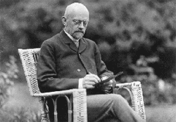
(Btw. the photo of James Glimm above was taken by George Bergman in 1972)

Comments closed

Quiver Grassmannians can be anything

Published May 2, 2013 by lieven

A standard Grassmannian $G r (m, V)$ is the manifold having as its points all possible $m$ -dimensional subspaces of a given vectorspace $V$ . As an example, $G r (1, V)$ is the set of lines through the origin in $V$ and therefore is the projective space $P (V)$ . Grassmannians are among the nicest projective varieties, they are smooth and allow a cell decomposition.

A quiver $Q$ is just an oriented graph. Here’s an example

A representation $V$ of a quiver assigns a vector-space to each vertex and a linear map between these vertex-spaces to every arrow. As an example, a representation $V$ of the quiver $Q$ consists of a triple of vector-spaces $(V_{1}, V_{2}, V_{3})$ together with linear maps $f_{a} : V_{2} \to V_{1}$ and $f_{b}, f_{c} : V_{2} \to V_{3}$ .

A sub-representation $W \subset V$ consists of subspaces of the vertex-spaces of $V$ and linear maps between them compatible with the maps of $V$ . The dimension-vector of $W$ is the vector with components the dimensions of the vertex-spaces of $W$ .

This means in the example that we require $f_{a} (W_{2}) \subset W_{1}$ and $f_{b} (W_{2})$ and $f_{c} (W_{2})$ to be subspaces of $W_{3}$ . If the dimension of $W_{i}$ is $m_{i}$ then $m = (m_{1}, m_{2}, m_{3})$ is the dimension vector of $W$ .

The quiver-analogon of the Grassmannian $G r (m, V)$ is the Quiver Grassmannian $Q G r (m, V)$ where $V$ is a quiver-representation and $Q G r (m, V)$ is the collection of all possible sub-representations $W \subset V$ with fixed dimension-vector $m$ . One might expect these quiver Grassmannians to be rather nice projective varieties.

However, last week Markus Reineke posted a 2-page note on the arXiv proving that every projective variety is a quiver Grassmannian.

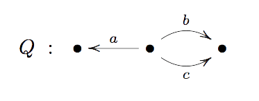
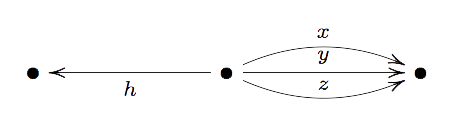
Let’s illustrate the argument by finding a quiver Grassmannian $Q G r (m, V)$ isomorphic to the elliptic curve in $P^{2}$ with homogeneous equation $Y^{2} Z = X^{3} + Z^{3}$ .

Consider the Veronese embedding $P^{2} \to P^{9}$ obtained by sending a point $(x : y : z)$ to the point

$(x^{3} : x^{2} y : x^{2} z : x y^{2} : x y z : x z^{2} : y^{3} : y^{2} z : y z^{2} : z^{3})$

The upshot being that the elliptic curve is now realized as the intersection of the image of $P^{2}$ with the hyper-plane $V (X_{0} - X_{7} + X_{9})$ in the standard projective coordinates $(x_{0} : x_{1} : \dots : x_{9})$ for $P^{9}$ .

To describe the equations of the image of $P^{2}$ in $P^{9}$ consider the $6 \times 3$ matrix with the rows corresponding to $(x^{2}, x y, x z, y^{2}, y z, z^{2})$ and the columns to $(x, y, z)$ and the entries being the multiplications, that is

$[\begin{matrix} x^{3} & x^{2} y & x^{2} z \\ x^{2} y & x y^{2} & x y z \\ x^{2} z & x y z & x z^{2} \\ x y^{2} & y^{3} & y^{2} z \\ x y z & y^{2} z & y z^{2} \\ x z^{2} & y z^{2} & z^{3} \end{matrix}] = [\begin{matrix} x_{0} & x_{1} & x_{2} \\ x_{1} & x_{3} & x_{4} \\ x_{2} & x_{4} & x_{5} \\ x_{3} & x_{6} & x_{7} \\ x_{4} & x_{7} & x_{8} \\ x_{5} & x_{8} & x_{9} \end{matrix}]$

But then, a point $(x_{0} : x_{1} : \dots : x_{9})$ belongs to the image of $P^{2}$ if (and only if) the matrix on the right-hand side has rank $1$ (that is, all its $2 \times 2$ minors vanish). Next, consider the quiver

and consider the representation $V = (V_{1}, V_{2}, V_{3})$ with vertex-spaces $V_{1} = C$ , $V_{2} = C^{10}$ and $V_{2} = C^{6}$ . The linear maps $x, y$ and $z$ correspond to the columns of the matrix above, that is

$(x_{0}, x_{1}, x_{2}, x_{3}, x_{4}, x_{5}, x_{6}, x_{7}, x_{8}, x_{9}) {\begin{cases} \to^{x} (x_{0}, x_{1}, x_{2}, x_{3}, x_{4}, x_{5}) \\ \to^{y} (x_{1}, x_{3}, x_{4}, x_{6}, x_{7}, x_{8}) \\ \to^{z} (x_{2}, x_{4}, x_{5}, x_{7}, x_{8}, x_{9}) \end{cases}$

The linear map $h : C^{10} \to C$ encodes the equation of the hyper-plane, that is $h = x_{0} - x_{7} + x_{9}$ .

Now consider the quiver Grassmannian $Q G r (m, V)$ for the dimension vector $m = (0, 1, 1)$ . A base-vector $p = (x_{0}, \dots, x_{9})$ of $W_{2} = C p$ of a subrepresentation $W = (0, W_{2}, W_{3}) \subset V$ must be such that $h (x) = 0$ , that is, $p$ determines a point of the hyper-plane.

Likewise the vectors $x (p), y (p)$ and $z (p)$ must all lie in the one-dimensional space $W_{3} = C$ , that is, the right-hand side matrix above must have rank one and hence $p$ is a point in the image of $P^{2}$ under the Veronese.

That is, $G r (m, V)$ is isomorphic to the intersection of this image with the hyper-plane and hence is isomorphic to the elliptic curve.

The general case is similar as one can view any projective subvariety $X \to P^{n}$ as isomorphic to the intersection of the image of a specific $d$ -uple Veronese embedding $P^{n} \to P^{N}$ with a number of hyper-planes in $P^{N}$ .

ADDED For those desperate to read the original comments-section, here’s the link.

Comments closed

The empty set according to bourbaki

Published February 9, 2013 by lieven

The footnote on page E. II.6 in Bourbaki’s 1970 edition of “Theorie des ensembles” reads

If this is completely obvious to you, stop reading now and start getting a life. For the rest of us, it took me quite some time before i was able to parse this formula, and when i finally did, it only added to my initial confusion.

Though the Bourbakis had a very preliminary version of their set-theory already out in 1939 (Fascicule des Resultats), the version as we know it now was published, chapter-wise, in the fifties: Chapters I and II in 1954, Chapter III in 1956 and finally Chapter IV in 1957.

In the first chapter they develop their version of logic, using ‘assemblages’ (assemblies) which are words of signs and letters, the signs being $τ, ◻, \lor, \neg, =, \in$ and $\supset$ .

Of these, we have the familiar signs $\lor$ (or), $\neg$ (not), $=$ (equal to) and $\in$ (element of) and, three more exotic ones: $τ$ (their symbol for the Hilbert operator $ε$ ), $◻$ a sort of wildcard variable bound by an occurrence of $τ$ (the ‘links’ in the above scan) and $\supset$ for an ordered couple.

The connectives are written in front of the symbols they connect rather than between them, avoiding brackets, so far example $(x \in y) \lor (x = x)$ becomes $\lor ϵ x y = x x$ .

If $R$ is some assembly and $x$ a letter occurring in $R$ , then the intende meaning of the *Hilbert-operator* $τ_{x} (R)$ is ‘some $x$ for which $R$ is true if such a thing exists’. $τ_{x} (R)$ is again an assembly constructed in three steps: (a) form the assembly $τ R$ , (b) link the starting $τ$ to all occurrences of $x$ in $R$ and (c) replace those occurrences of $x$ by an occurrence of $◻$ .

For MathJax reasons we will not try to draw links but rather give a linked $τ$ and $◻$ the same subscript. So, for example, the claimed assembly for $\emptyset$ above reads

$τ_{y} \neg \neg \neg \in τ_{x} \neg \neg \in ◻_{x} ◻_{y} ◻_{y}$

If $A$ and $B$ are assemblies and $x$ a letter occurring in $B$ then we denote by $(A | x) B$ the assembly obtained by replacing each occurrence of $x$ in $B$ by the assembly $A$ . The upshot of this is that we can now write quantifiers as assemblies:

$(\exists x) R$ is the assembly $(τ_{x} (R) | x) R$ and as $(\forall x) R$ is $\neg (\exists x) \neg R$ it becomes $\neg (τ_{x} (\neg R) | x) \neg R$

Okay, let’s try to convert Bourbaki’s definition of the emptyset $\emptyset$ as ‘something that contains no element’, or formally $τ_{y} ((\forall x) (x \notin y))$ , into an assembly.

– by definition of $\forall$ it becomes $τ_{y} (\neg (\exists x) (\neg (x \notin y)))$
– write $\neg (x \notin y)$ as the assembly $R = \neg \neg \in x ◻_{y}$
– then by definition of $\exists$ we have to assemble $τ_{y} \neg (τ_{x} (R) | x) R$
– by construction $τ_{x} (R) = τ_{x} \neg \neg \in ◻_{x} ◻_{y}$
– using the description of $(A | x) B$ we finally indeed obtain $τ_{y} \neg \neg \neg \in τ_{x} \neg \neg \in ◻_{x} ◻_{y} ◻_{y}$

But, can someone please explain what’s wrong with $τ_{y} \neg \in τ_{x} \in ◻_{x} ◻_{y} ◻_{y}$ which is the assembly corresponding to $τ_{y} (\neg (\exists x) (x \in y))$ which could equally well have been taken as defining the empty set and has a shorter assembly (length 8 and 3 links, compared to the one given of length 12 with 3 links).

Hair-splitting as this is, it will have dramatic implications when we will try to assemble Bourbaki’s definition of “1” another time.

Comments closed

Category: math

A noncommutative moduli space

Quiver Grassmannians can be anything

The empty set according to bourbaki