Category: geometry

Connes-Consani for undergraduates (1)

Published October 3, 2008 by lieven

A couple of weeks ago, Alain Connes and Katia Consani arXived their paper “On the notion of geometry over $\mathbb{F}_1 $”. Their subtle definition is phrased entirely in Grothendieck‘s scheme-theoretic language of representable functors and may be somewhat hard to get through if you only had a few years of mathematics.

I’ll try to give the essence of their definition of an affine scheme over $\mathbb{F}_1 $ (and illustrate it with an example) in a couple of posts. All you need to know is what a finite Abelian group is (if you know what a cyclic group is that’ll be enough) and what a commutative algebra is. If you already know what a functor and a natural transformation is, that would be great, but we’ll deal with all that abstract nonsense when we’ll need it.

So take two finite Abelian groups A and B, then a group-morphism is just a map $f~:~A \rightarrow B $ preserving the group-data. That is, f sends the unit element of A to that of B and
f sends a product of two elements in A to the product of their images in B. For example, if $A=C_n $ is a cyclic group of order n with generator g and $B=C_m $ is a cyclic group of order m with generator h, then every groupmorphism from A to B is entirely determined by the image of g let’s say that this image is $h^i $. But, as $g^n=1 $ and the conditions on a group-morphism we must have that $h^{in} = (h^i)^n = 1 $ and therefore m must divide i.n. This gives you all possible group-morphisms from A to B.

They are plenty of finite abelian groups and many group-morphisms between any pair of them and all this stuff we put into one giant sack and label it $\mathbf{abelian} $. There is another, even bigger sack, which is even simpler to describe. It is labeled $\mathbf{sets} $ and contains all sets as well as all maps between two sets.

Right! Now what might be a map $F~:~\mathbf{abelian} \rightarrow \mathbf{sets} $ between these two sacks? Well, F should map any abelian group A to a set F(A) and any group-morphism $f~:~A \rightarrow B $ to a map between the corresponding sets $F(f)~:~F(A) \rightarrow F(B) $ and do all of this nicely. That is, F should send compositions of group-morphisms to compositions of the corresponding maps, and so on. If you take a pen and a piece of paper, you’re bound to come up with the exact definition of a functor (that’s what F is called).

You want an example? Well, lets take F to be the map sending an Abelian group A to its set of elements (also called A) and which sends a groupmorphism $A \rightarrow B $ to the same map from A to B. All F does is ‘forget’ the extra group-conditions on the sets and maps. For this reason F is called the forgetful functor. We will denote this particular functor by $\underline{\mathbb{G}}_m $, merely to show off.

Luckily, there are lots of other and more interesting examples of such functors. Our first class we will call maxi-functors and they are defined using a finitely generated $\mathbb{C} $-algebra R. That is, R can be written as the quotient of a polynomial algebra

$R = \frac{\mathbb{C}[x_1,\ldots,x_d]}{(f_1,\ldots,f_e)} $

by setting all the polynomials $f_i $ to be zero. For example, take R to be the ring of Laurant polynomials

$R = \mathbb{C}[x,x^{-1}] = \frac{\mathbb{C}[x,y]}{(xy-1)} $

Other, and easier, examples of $\mathbb{C} $-algebras is the group-algebra $\mathbb{C} A $ of a finite Abelian group A. This group-algebra is a finite dimensional vectorspace with basis $e_a $, one for each element $a \in A $ with multiplication rule induced by the relations $e_a.e_b = e_{a.b} $ where on the left-hand side the multiplication . is in the group-algebra whereas on the right hand side the multiplication in the index is that of the group A. By choosing a different basis one can show that the group-algebra is really just the direct sum of copies of $\mathbb{C} $ with component-wise addition and multiplication

$\mathbb{C} A = \mathbb{C} \oplus \ldots \oplus \mathbb{C} $

with as many copies as there are elements in the group A. For example, for the cyclic group $C_n $ we have

$\mathbb{C} C_n = \frac{\mathbb{C}[x]}{(x^n-1)} = \frac{\mathbb{C}[x]}{(x-1)} \oplus \frac{\mathbb{C}[x]}{(x-\zeta)} \oplus \frac{\mathbb{C}[x]}{(x-\zeta^2)} \oplus \ldots \oplus \frac{\mathbb{C}[x]}{(x-\zeta^{n-1})} = \mathbb{C} \oplus \mathbb{C} \oplus \mathbb{C} \oplus \ldots \oplus \mathbb{C} $

The maxi-functor asociated to a $\mathbb{C} $-algebra R is the functor

$\mathbf{maxi}(R)~:~\mathbf{abelian} \rightarrow \mathbf{sets} $

which assigns to a finite Abelian group A the set of all algebra-morphism $R \rightarrow \mathbb{C} A $ from R to the group-algebra of A. But wait, you say (i hope), we also needed a functor to do something on groupmorphisms $f~:~A \rightarrow B $. Exactly, so to f we have an algebra-morphism $f’~:~\mathbb{C} A \rightarrow \mathbb{C}B $ so the functor on morphisms is defined via composition

$\mathbf{maxi}(R)(f)~:~\mathbf{maxi}(R)(A) \rightarrow \mathbf{maxi}(R)(B) \qquad \phi~:~R \rightarrow \mathbb{C} A \mapsto f’ \circ \phi~:~R \rightarrow \mathbb{C} A \rightarrow \mathbb{C} B $

So, what is the maxi-functor $\mathbf{maxi}(\mathbb{C}[x,x^{-1}] $? Well, any $\mathbb{C} $-algebra morphism $\mathbb{C}[x,x^{-1}] \rightarrow \mathbb{C} A $ is fully determined by the image of $x $ which must be a unit in $\mathbb{C} A = \mathbb{C} \oplus \ldots \oplus \mathbb{C} $. That is, all components of the image of $x $ must be non-zero complex numbers, that is

$\mathbf{maxi}(\mathbb{C}[x,x^{-1}])(A) = \mathbb{C}^* \oplus \ldots \oplus \mathbb{C}^* $

where there are as many components as there are elements in A. Thus, the sets $\mathbf{maxi}(R)(A) $ are typically huge which is the reason for the maxi-terminology.

Next, let us turn to mini-functors. They are defined similarly but this time using finitely generated $\mathbb{Z} $-algebras such as $S=\mathbb{Z}[x,x^{-1}] $ and the integral group-rings $\mathbb{Z} A $ for finite Abelian groups A. The structure of these inegral group-rings is a lot more delicate than in the complex case. Let’s consider them for the smallest cyclic groups (the ‘isos’ below are only approximations!)

$\mathbb{Z} C_2 = \frac{\mathbb{Z}[x]}{(x^2-1)} = \frac{\mathbb{Z}[x]}{(x-1)} \oplus \frac{\mathbb{Z}[x]}{(x+1)} = \mathbb{Z} \oplus \mathbb{Z} $

$\mathbb{Z} C_3 = \frac{\mathbb{Z}[x]}{(x^3-1)} = \frac{\mathbb{Z}[x]}{(x-1)} \oplus \frac{\mathbb{Z}[x]}{(x^2+x+1)} = \mathbb{Z} \oplus \mathbb{Z}[\rho] $

$\mathbb{Z} C_4 = \frac{\mathbb{Z}[x]}{(x^4-1)} = \frac{\mathbb{Z}[x]}{(x-1)} \oplus \frac{\mathbb{Z}[x]}{(x+1)} \oplus \frac{\mathbb{Z}[x]}{(x^2+1)} = \mathbb{Z} \oplus \mathbb{Z} \oplus \mathbb{Z}[i] $

For a $\mathbb{Z} $-algebra S we can define its mini-functor to be the functor

$\mathbf{mini}(S)~:~\mathbf{abelian} \rightarrow \mathbf{sets} $

which assigns to an Abelian group A the set of all $\mathbb{Z} $-algebra morphisms $S \rightarrow \mathbb{Z} A $. For example, for the algebra $\mathbb{Z}[x,x^{-1}] $ we have that

$\mathbf{mini}(\mathbb{Z} [x,x^{-1}]~(A) = (\mathbb{Z} A)^* $

the set of all invertible elements in the integral group-algebra. To study these sets one has to study the units of cyclotomic integers. From the above decompositions it is easy to verify that for the first few cyclic groups, the corresponding sets are $\pm C_2, \pm C_3 $ and $\pm C_4 $. However, in general this set doesn’t have to be finite. It is a well-known result that the group of units of an integral group-ring of a finite Abelian group is of the form

$(\mathbb{Z} A)^* = \pm A \times \mathbb{Z}^{\oplus r} $

where $r = \frac{1}{2}(o(A) + 1 + n_2 -2c) $ where $o(A) $ is the number of elements of A, $n_2 $ is the number of elements of order 2 and c is the number of cyclic subgroups of A. So, these sets can still be infinite but at least they are a lot more manageable, explaining the mini-terminology.

Now, we would love to go one step deeper and define nano-functors by the same procedure, this time using finitely generated algebras over $\mathbb{F}_1 $, the field with one element. But as we do not really know what we might mean by this, we simply define a nano-functor to be a subfunctor of a mini-functor, that is, a nano-functor N has an associated mini-functor $\mathbf{mini}(S) $ such that for all finite Abelian groups A we have that $N(A) \subset \mathbf{mini}(S)(A) $.

For example, the forgetful functor at the beginning, which we pompously denoted $\underline{\mathbb{G}}_m $ is a nano-functor as it is a subfunctor of the mini-functor $\mathbf{mini}(\mathbb{Z}[x,x^{-1}]) $.

Now we are allmost done : an affine $\mathbb{F}_1 $-scheme in the sense of Connes and Consani is a pair consisting of a nano-functor N and a maxi-functor $\mathbf{maxi}(R) $ such that two rather strong conditions are satisfied :

there is an evaluation ‘map’ of functors $e~:~N \rightarrow \mathbf{maxi}(R) $
this pair determines uniquely a ‘minimal’ mini-functor $\mathbf{mini}(S) $ of which N is a subfunctor

of course we still have to turn this into proper definitions but that will have to await another post. For now, suffice it to say that the pair $~(\underline{\mathbb{G}}_m,\mathbf{maxi}(\mathbb{C}[x,x^{-1}])) $ is a $\mathbb{F}_1 $-scheme with corresponding uniquely determined mini-functor $\mathbf{mini}(\mathbb{Z}[x,x^{-1}]) $, called the multiplicative group scheme.

Continued here

F_un with Manin

Published September 10, 2008 by lieven

Amidst all LHC-noise, Yuri I. Manin arXived today an interesting paper Cyclotomy and analytic geometry over $\mathbb{F}_1 $.

The paper gives a nice survey of the existent literature and focusses on the crucial role of roots of unity in the algebraic geometry over the non-existent field with one element $\mathbb{F}_1 $ (in French called ‘F-un’). I have tried to do a couple of posts on F-un some time ago but now realize, reading Manin’s paper, I may have given up way too soon…

At several places in the paper, Manin hints at a possible noncommutative geometry over $\mathbb{F}_1 $ :

This is the appropriate place to stress that in a wider context of Toen-Vaqui ‘Au-dessous de Spec Z’, or eventually in noncommutative $\mathbb{F}_1 $-geometry, teh spectrum of $\mathbb{F}_1 $ loses its privileged position as a final object of a geometric category. For example, in noncommutative geometry, or in an appropriate category of stacks, the quotient of this spectrum modulo the trivial action of a group must lie below this spectrum.

Soule’s algebras $\mathcal{A}_X $ are a very important element of the structure, in particular, because they form a bridge to Arakelov geometry. Soule uses concrete choices of them in order to produce ‘just right’ supply of morphisms, without a priori constraining these choices formally. In this work, we use these algebras and their version also to pave a way to the analytic (and possibly non-commutative) geometry over $\mathbb{F}_1 $.

Back when I was writing the first batch of F-un posts, I briefly contemplated the possibility of a noncommutative geometry over $\mathbb{F}_1 $, but quickly forgot about it because I thought it would be forced to reduce to commutative geometry.

Here is the quick argument : noncommutative geometry is really the study of coalgebras (see for example my paper or if you prefer more trustworthy sources the Kontsevich-Soibelman paper). Now, unless I made a mistake, I think all coalgebras over $\mathbb{F}_1 $ must be co-commutative (even group-like), so reducing to commutative geometry.

Surely, I’m missing something…

the buckyball curve

Published July 2, 2008 by lieven

We are after the geometric trinity corresponding to the trinity of exceptional Galois groups

The surfaces on the right have the corresponding group on the left as their group of automorphisms. But, there is a lot more group-theoretic info hidden in the geometry. Before we sketch the $L_2(11) $ case, let us recall the simpler situation of $L_2(7) $.

There are some excellent web-page on the Klein quartic and it would be too hard to try to improve on them, so we refer to John Baez’ page and Greg Egan’s page for more details.

The Klein quartic is the degree 4 projective plane curve defined by the equation $x^3y+y^3z+z^3x=0 $. It can be tiled with a set of 24 regular heptagons, or alternatively with a set of 56 equilateral triangles and these two tilings are dual to each other

In the triangular tiling, there are 56 triangles, 84 edges and 24 vertices. The 56 triangles come in 7 bunches of 8 each and we give the 7 bunches of triangles each a different color as in the pictures below made by Greg Egan. Observe that in the hyperbolic tiling all triangles look alike, but in the picture on the left most of them get warped as we try to embed the quartic in 3-space (which is impossible to do properly). The non-warped triangles (the red ones) come into pairs, the top and bottom triangles of a triangular prism, one prism at each of the four ‘vertices’ of a tetrahedron.

The automorphism group $L_2(7) $ acts on these triangles as $S_4 $ acts on the triangles in a truncated cube.

The buckyball construction from a conjugacy class of order 11 elements from $L_2(11) $ recalled last time, has an analogon $L_2(7) $, leading to the truncated cube.

In $L_2(7) $ there are two conjugacy classes of subgroups isomorphic to $S_4 $ (the rotation-symmetry group of the cube) as well as two conjugacy classes of order 7 elements, each consisting of precisely 24 elements, say C and D. The normalizer subgroup of C has order 21, so there is a cyclic group of order 3 acting non-trivially on the conjugacy class C with 8 orbits consisting of three elements each. These are the eight triangles of the truncated cube identified above as the red triangles.

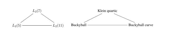
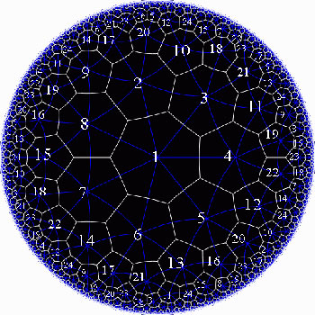
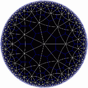
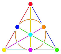Shifting perspective, we can repeat this for each of the seven different colors. That is, we have seven truncated cubes in the Klein quartic. On each of them a copy of $S_4 $ acts and these subgroups form one of the two conjugacy classes of $S_4 $ in the group $L_2(7) $. The colors of the triangles of these seven truncated cubes are indicated by bullets in the picture above on the right. The other conjugacy class of $S_4 $’s act on ‘truncated anti-cubes’ which also come in seven bunches of which the color is indicated by a square in that picture.

If you spend enough time on it you will see that each (truncated) cube is completely disjoint from precisely 3 (truncated) anti-cubes. This reminds us of the Fano-plane (picture on the left) : it has 7 points (our seven truncated cubes), 7 lines (the truncated anti-cubes) and the incidence relation of points and lines corresponds to the disjointness of (truncated) cubes and anti-cubes! This is the geometric interpretation of the group-theoretic realization that $L_2(7) \simeq PGL_3(\mathbb{F}_2) $ is the isomorphism group of the projective plane over the finite field $\mathbb{F}_2 $ on two elements, that is, the Fano plane. The colors of the picture on the left indicate the colors of cubes (points) and anti-cubes (lines) consistent with Egan’s picture above.

Further, the 24 vertices correspond to the 24 cusps of the modular group $\Gamma(7) $. Recall that a modular interpretation of the Klein quartic is as $\mathbb{H}/\Gamma(7) $ where $\mathbb{H} $ is the upper half-plane on which the modular group $\Gamma = PSL_2(\mathbb{Z}) $ acts via Moebius transformations, that is, to a 2×2 matrix corresponds the transformation

[tex]\begin{bmatrix} a & b \\ c & d \end{bmatrix}[/tex] <----> $ z \mapsto \frac{az+b}{cz+d} $

Okay, now let’s briefly sketch the exciting results found by Pablo Martin and David Singerman in the paper From biplanes to the Klein quartic and the buckyball, extending the above to the group $L_2(11) $.

There is one important modification to be made. Recall that the Cayley-graph to get the truncated cube comes from taking as generators of the group $S_4 $ the set ${ (3,4),(1,2,3) } $, that is, an order two and an order three element, defining an epimorphism from the modular group $\Gamma= C_2 \ast C_3 \rightarrow S_4 $.

We have also seen that in order to get the buckyball as a Cayley-graph for $A_5 $ we need to take the generating set ${ (2,3)(4,5),(1,2,3,4,5) } $, so a degree two and a degree five element.

Hence, if we want to have a corresponding Riemann surface we’d better not start from the action of the modular group on the upper half-plane, but rather the action via Moebius transformations of the
Hecke group

$H^5 \simeq C_2 \ast C_5 = \langle z \mapsto -\frac{1}{z}, z \mapsto z+ \phi \rangle $

where $\phi = \frac{1 + \sqrt{5}}{2} $ is the golden ratio.

But then, there is an epimorphism $H^5 \rightarrow L_2(11) $ (as this group is generated by one element of degree 2 and one of degree 5) and let $\Lambda $ denote its kernel. Observe that $\Lambda $ is the analogon of the modular subgroup $\Gamma(7) $ used above to define the Klein quartic.

Hence, Martin and Singerman define the buckyball curve as the modular quotient $X=\mathbb{H}/\Lambda $ which is a Riemann surface of genus 70.

The terminlogy is motivated by the fact that, precisely as we got 7 truncated cubes in the Klein quartic, we now get 11 truncated icosahedra (that is, buckyballs) in $X $. The 11 coming, analogous to the Klein case, from thefact that there are precisely two conjugacy classes of subgroups of $L_2(11) $ isomorphic to $A_5 $, each class containing precisely eleven elements!
The 60 vertices of the buckyball again correspond to the fact that there are 60 cusps in this case.

So, what is the analogon of the Fano plane in this case? Well, observe that the Fano-plane is a biplane of order two. That is, if we take as ‘points’ the points of the Fano plane and as ‘lines’ the complements of lines in the Fano plane then this defines a biplane structure. This means that any two distinct ‘points’ are contained in two distinct ‘lines’ and that two distinct ‘lines’ intersect in two distinct ‘points’. A biplane is said to be of order k is each ‘line’ consist of k-2 ‘points’. As the complement of a line in the Fano plane consists of 4 points, the Fano plane is therefore a biplane of order 2. The intersection pattern of cubes and anti-cubes in the Klein quartic is this biplane structure on the Fano plane.

In a similar way, Martin and Singerman show that the two conjugacy classes of subgroups isomorphic to $A_5 $ in $L_2(11) $, each containing exactly 11 elements, correspond to 11 embedded buckyballs (and 11 anti-buckyballs) in the buckyball-curve $X $ and that the intersection relations among them describe the combinatorial structure of a biplane of order three if we view the 11 buckys as ‘points’ and the anti-buckys as ‘lines’.

That is, the buckyball curve is a perfect geometric counterpart of the Klein quartic for the two trinities

At the Arcadian Functor, Kea also has a post on this in which she conjectures that the Kac-Moody algebra of E11 may be related to the buckyball curve.

References :

David Singerman, “Klein’s Riemann surface of genus 3 and regular embeddings of finite projective planes” Bull. London Math. Soc. 18 (1986) 364-370.

Pablo Martin and David Singerman, “From biplanes to the Klein quartic and the Buckyball” (note that this is a preliminary version, please contact David Singerman for the latest version).