A comment-thread well worth following while on vacation was Algebraic Geometry without Prime Ideals at the Secret Blogging Seminar. Peter Woit became lyric about it :
My nomination for the all-time highest quality discussion ever held in a blog comment section goes to the comments on this posting at Secret Blogging Seminar, where several of the best (relatively)-young algebraic geometers in the business discuss the foundations of the subject and how it should be taught.
I follow far too few comment-sections to make such a definite statement, but found the contributions by James Borger and David Ben-Zvi of exceptional high quality. They made a case for using Grothendieck’s ‘functor of points’ approach in teaching algebraic geometry instead of the ‘usual’ approach via prime spectra and their structure sheaves.
The text below was written on december 15th of last year, but never posted. As far as I recall it was meant to be part two of the ‘Brave New Geometries’-series starting with the Mumford’s treasure map post. Anyway, it may perhaps serve someone unfamiliar with Grothendieck’s functorial approach to make the first few timid steps in that directions.
 Allyn Jackson’s beautiful account of Grothendieck’s life “Comme Appele du Neant, part II” (the first part of the paper can be found here) contains this gem :
“One striking characteristic of Grothendieck’s
mode of thinking is that it seemed to rely so little
on examples. This can be seen in the legend of the
so-called “Grothendieck prime”.
In a mathematical
conversation, someone suggested to Grothendieck
that they should consider a particular prime number.
“You mean an actual number?” Grothendieck
asked. The other person replied, yes, an actual
prime number. Grothendieck suggested, “All right,
take 57.”
But Grothendieck must have known that 57 is not
prime, right? Absolutely not, said David Mumford
of Brown University. “He doesn’t think concretely.””
We have seen before how Mumford’s doodles allow us to depict all ‘points’ of the affine scheme $\mathbf{spec}(\mathbb{Z}[x]) $, that is, all prime ideals of the integral polynomial ring $\mathbb{Z}[x] $.
Perhaps not too surprising, in view of the above story, Alexander Grothendieck pushed the view that one should consider all ideals, rather than just the primes. He achieved this by associating the ‘functor of points’ to an affine scheme.
Consider an arbitrary affine integral scheme $X $ with coordinate ring $\mathbb{Z}[X] = \mathbb{Z}[t_1,\ldots,t_n]/(f_1,\ldots,f_k) $, then any ringmorphism
$\phi~:~\mathbb{Z}[t_1,\ldots,t_n]/(f_1,\ldots,f_k) \rightarrow R $
is determined by an n-tuple of elements $~(r_1,\ldots,r_n) = (\phi(t_1),\ldots,\phi(t_n)) $ from $R $ which must satisfy the polynomial relations $f_i(r_1,\ldots,r_n)=0 $. Thus, Grothendieck argued, one can consider $~(r_1,\ldots,r_n) $ an an ‘$R $-point’ of $X $ and all such tuples form a set $h_X(R) $ called the set of $R $-points of $X $. But then we have a functor
$h_X~:~\mathbf{commutative rings} \rightarrow \mathbf{sets} \qquad R \mapsto h_X(R)=Rings(\mathbb{Z}[t_1,\ldots,t_n]/(f_1,\ldots,f_k),R) $
So, what is this mysterious functor in the special case of interest to us, that is when $X = \mathbf{spec}(\mathbb{Z}[x]) $?
Well, in that case there are no relations to be satisfied so any ringmorphism $\mathbb{Z}[x] \rightarrow R $ is fully determined by the image of $x $ which can be any element $r \in R $. That is, $Ring(\mathbb{Z}[x],R) = R $ and therefore Grothendieck’s functor of points
$h_{\mathbf{spec}(\mathbb{Z}[x]} $ is nothing but the forgetful functor.
But, surely the forgetful functor cannot give us interesting extra information on Mumford’s drawing?
Well, have a look at the slightly extended drawing below :
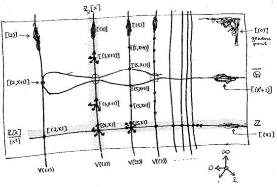
What are these ‘smudgy’ lines and ‘spiky’ points? Well, before we come to those let us consider the easier case of identifying the $R $-points in case $R $ is a domain. Then, for any $r \in R $, the inverse image of the zero prime ideal of $R $ under the ringmap $\phi_r~:~\mathbb{Z}[x] \rightarrow R $ must be a prime ideal of $\mathbb{Z}[x] $, that is, something visible in Mumford’s drawing. Let’s consider a few easy cases :
 For starters, what are the $\mathbb{Z} $-points of $\mathbf{spec}(\mathbb{Z}[x]) $? Any natural number $n \in \mathbb{Z} $ determines the surjective ringmorphism $\phi_n~:~\mathbb{Z}[x] \rightarrow \mathbb{Z} $ identifying $\mathbb{Z} $ with the quotient $\mathbb{Z}[x]/(x-n) $, identifying the ‘arithmetic line’ $\mathbf{spec}(\mathbb{Z}) = { (2),(3),(5),\ldots,(p),\ldots, (0) } $ with the horizontal line in $\mathbf{spec}(\mathbb{Z}[x]) $ corresponding to the principal ideal $~(x-n) $ (such as the indicated line $~(x) $).
When $\mathbb{Q} $ are the rational numbers, then $\lambda = \frac{m}{n} $ with $m,n $ coprime integers, in which case we have $\phi_{\lambda}^{-1}(0) = (nx-m) $, hence we get again an horizontal line in $\mathbf{spec}(\mathbb{Z}[x]) $. For $ \overline{\mathbb{Q}} $, the algebraic closure of $\mathbb{Q} $ we have for any $\lambda $ that $\phi_{\lambda}^{-1}(0) = (f(x)) $ where $f(x) $ is a minimal integral polynomial for which $\lambda $ is a root.
But what happens when $K = \mathbb{C} $ and $\lambda $ is a trancendental number? Well, in that case the ringmorphism $\phi_{\lambda}~:~\mathbb{Z}[x] \rightarrow \mathbb{C} $ is injective and therefore $\phi_{\lambda}^{-1}(0) = (0) $ so we get the whole arithmetic plane!
In the case of a finite field $\mathbb{F}_{p^n} $ we have seen that there are ‘fat’ points in the arithmetic plane, corresponding to maximal ideals $~(p,f(x)) $ (with $f(x) $ a polynomial of degree $n $ which remains irreducible over $\mathbb{F}_p $), having $\mathbb{F}_{p^n} $ as their residue field. But these are not the only $\mathbb{F}_{p^n} $-points. For, take any element $\lambda \in \mathbb{F}_{p^n} $, then the map $\phi_{\lambda} $ takes $\mathbb{Z}[x] $ to the subfield of $\mathbb{F}_{p^n} $ generated by $\lambda $. That is, the $\mathbb{F}_{p^n} $-points of $\mathbf{spec}(\mathbb{Z}[x]) $ consists of all fat points with residue field $\mathbb{F}_{p^n} $, together with slightly slimmer points having as their residue field $\mathbb{F}_{p^m} $ where $m $ is a divisor of $n $. In all, there are precisely $p^n $ (that is, the number of elements of $\mathbb{F}_{p^n} $) such points, as could be expected.
Things become quickly more interesting when we consider $R $-points for rings containing nilpotent elements.
Comments closed The
The  Last week,
  6-dimensional quadrics may be quite hard to visualize, so it may help to recall the classic situation of lines on a 2-dimensional quadric (animated gif taken from
  To see this, note that the automorphism group of a 6-dimensional smooth quadric is the rotation group $SO_8(\mathbb{C}) $ and this group has