Around 1975 Sir Roger Penrose discovered his aperiodic P2 tilings of the plane, using only two puzzle pieces: Kites (K) and Darts (D)
The inner angles of these pieces are all multiples of $36^o = \tfrac{180^o}{5}$, the short edges have length $1$, and the long edges have length $\tau = \tfrac{1+\sqrt{5}}{2}$, the golden ratio. These pieces must be joined together so that the colours match up (if we do not use this rule it is easy to get periodic tilings with these two pieces).
There is plenty of excellent online material available:
- The two original Martin Gardner Scientific American articles on Penrose tiles have been made available by the MAA, and were reprinted in “Penrose Tiles to Trapdoor Ciphers”. They contain most of Conway’s early discoveries about these tilings, but without proofs.
- A JavaScript application by Kevin Bertman to play around with these tilings. You can deflate and inflate tilings, find forced tiles and much more. Beneath the app-window there’s a detailed explanation of all the basics, including inflation and deflation of the P2-tiles, the seven types of local vertex configurations (naming by Conway, of course),
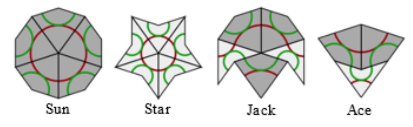
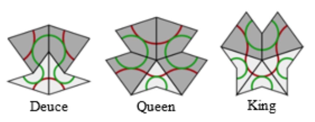
proofs of aperiodicity (similar to the one for Conway’s musical sequences), that every tile lies within an ace (similar to the LSL-subword in musical sequences) with application to local isomorphism (again similar to the $1$-dimensional case).
- Course notes of an Oxford masterclass in geometry Lectures on Penrose tilings by Alexander Ritter, again with proofs of all of the above and a discussion about the Cartwheel tilings (similar to that in the post on musical sequences), giving an algorithm to decide whether or not a partial tiling can be extended to the entire plane, or not.
There’s no point copying this material here. Rather, I’d like to use some time in this GoV series of posts to talk about de Bruijn’s pentagrid results. For this reason, I now need to make the connection with Penrose’s ‘other’ tilings, the P3 tiles of ‘thin’ and ‘thick’ rhombi (sometimes called ‘skinny’ and ‘fat’ rhombi).
Every Penrose P2-tiling can be turned into a P3-rhombic tiling, and conversely.
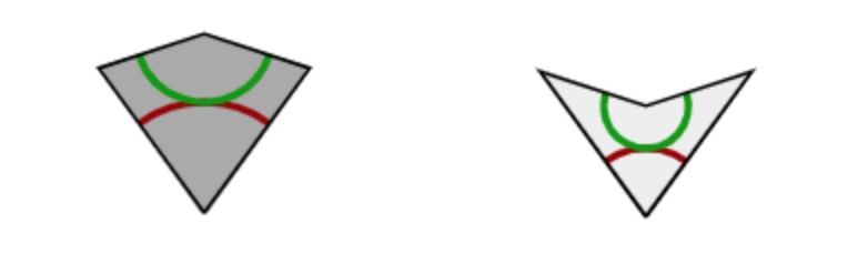
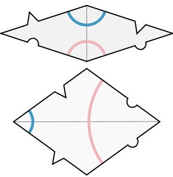
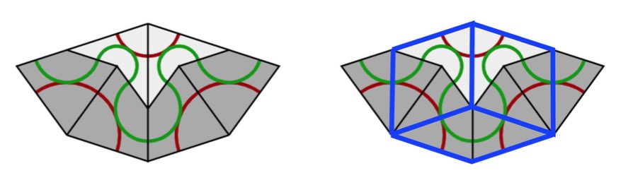
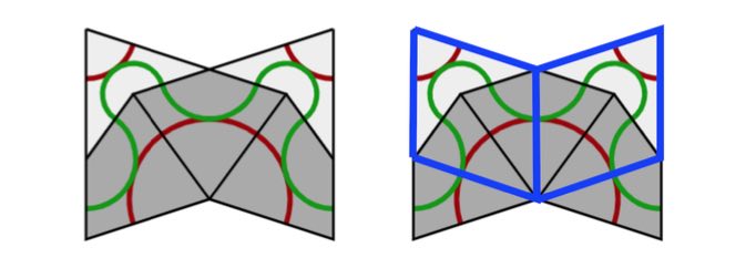
From kites and darts to rhombi: divide every kite in two halves along its line of reflection. Then combine darts and half-kites into rhombi where a fat rhombus consists of a dart and two half-kites, joined at a long edge, and a skinny rhombus is made of two half-kites, joined at a short edge. This can always be done preserving the gluing conditions. It suffices to verify this for the deflated kite and dart (on the left below) and we see that the matching colour-conditions are those of the rhombi.
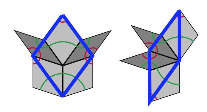
From rhombi to kites and darts: divide every fat rhombus into a dart (placed at the red acute angle) and two half-kites, joined at a long edge, and divide every skinny rhombus into two half-kites along its short diagonal.
All results holding for Kites and Darts tilings have therefore their versions for Rhombic tilings. For example, we have rhombic deflation and inflation rules
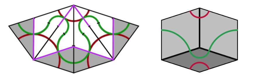
A Rhombic tiling can be seen as an intermediate step in the inflation process of a Penrose tiling $P$. Start by dividing all kites in two halves along their long diagonal and all darts in two halves along their short diagonal (the purple lines below).
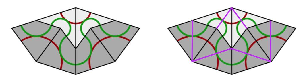
If we consider all original black lines together with the new purple ones, we get a tiling of the plane by triangles and we call this the $A$-tiling. There are two triangles, s small triangle $S_A$ (the whiter ones, with two small edges ofd length $1$ and one edge of length $\tau$) and a large triangle $L_A$ (the greyer ones, with two edges of length $\tau$ and one edge of length $1$).
Next, we remove the black lines joining an $S_A$-triangle with an $L_A$-triangle, and get another tiling with triangles, the $B$-tiling, with two pieces, a large triangle $L_B$ with two sides of length $\tau$ and one side of length $1+\tau$ (the white ones) (the union of an $L_A$ and a $S_A$), and a small triangle $S_B$ which has the same form as $L_A$ (the greyer ones). If we now join two white triangles $L_B$ along their common longer edge, and two greyer triangles $S_B$ along their common smaller edge, we obtain the Rhombic tiling $R$ corresponding to $P$.
We can repeat this process starting with the Rhombic tiling $R$. We divide all fat rhombi in two along their long diagonals, and the skinny rhombi in two along their short diagonals (the purple lines). We obtain a tiling of the plane by triangles, which is of course just the $B$-tiling above.
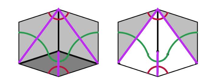
Remove the edge joining a small $S_B$ with a large $L_B$ triangle, then we get a new tiling by triangles, the $\tau A$-tiling consisting of large triangles $L_{\tau A}$ (the white ones) with two long edges of length $1+\tau$ and one short edge of length $\tau$ (note that $L_{\tau A}$ is $\tau$ times the triangle $L_A$), and a smaller one $S_{\tau A}$ (the grey ones) having two short edges of length $\tau$ and one long edge of length $1+\tau$ (again $S_{\tau A}$ is $\tau$ times the triangle $S_A$). If we join two $L_{\tau A}$-triangles sharing a common long edge we obtain a Kite ($\tau$-times larger than the original Kite) and if we joint two $S_{\tau A}$-triangles along their common small edge we get a Dart ($\tau$ times larger than the original Dart). The Penrose tiling we obtain is the inflation $inf(P)$ of the original $P$.
If we repeat the whole procedure starting from $inf(P)$ instead of $P$ we get, in turn, triangle tilings of the plane, subsequently the $\tau B$-tiling, the $\tau^2 A$-tiling, the $\tau^2 B$-tiling and so on, the triangles in a $\tau^n A$-tiling being of size $\tau^2$-times those of the $A$-tiling, and those in the $\tau^n B$-tiling $\tau^n$-times as large as those of the $B$-tiling.
The upshot of this is that we can associate to a Penrose tiling $P$ of the plane a sequence of $0$’s and $1$’s. Starting from $P$ we have an infinite sequence of associated triangle tilings
\[
A,~B,~\tau A,~\tau B,~\tau^2 A, \dots,~\tau^n A,~\tau^n B,~\tau^{n+1} A, \dots \]
with larger and larger triangle tiles. Let $p$ be a point of the plane lying in the interior of an $A$-tile, then we define its index sequence
\[
i(P,p) = (x_0,x_1,x_2,\dots ) \quad x_{2n} = \begin{cases} 0~\text{if $p \in L_{\tau^n A}$} \\ 1~\text{if $p \in S_{\tau^n A}$} \end{cases}~ x_{2n+1} = \begin{cases} 0~\text{if $p \in L_{\tau^n B}$} \\ 1~\text{if $p \in S_{\tau^n B}$} \end{cases} \]
That is, $x_0=1$ if $p$ lies in a small triangle of the $A$-tiling and $x_0=1$ if it lies in a large triangle, $x_1=1$ if $p$ lies in a small triangle of the $B$-tiling and is $0$ if it lies in a large $B$-triangle, and so on.
The beauty of this is that every infinite sequence $(x_0,x_1,x_2,\dots )$ whose terms are $0$ or $1$, and in which no two consecutive terms are equal to $1$, is the index sequence $i(P,p)$ of some Penrose tiling $P$ in some point $p$ of the plane.
From the construction of the sequence of triangle-tilings it follows that a small triangle is part of a large triangle in the next tiling. For this reason an index sequence can never have two consecutive ones. An index sequence gives explicit instructions as to how the Penrose tiling is constructed. In each step add a large or small triangle as to fit the sequence, together with the matching triangle (the other half of a Penrose or Rhombic tile). Next, look at the patches $P_i$ of Kites and Darts (in the $\tau^i A$ tiling), for $i=0,1,\dots$, then $P_{i-k}$ is contained in the $k$-times inflated $P_i$, $i^k(P_i)$ (without rescaling), for each $i$ and all $1 \leq k \leq i$. But then, we have a concentric series of patches
\[
P_0 \subset i(P_1) \subset i^2(P_2) \subset \dots \]
filling the entire plane.

The index sequence depends on the choice of point $p$ in the plane. If $p’$ is another point, then as the triangle tiles increase is size at each step, $p$ and $p’$ will lie in the same triangle-tile at some stage, and after that moment their index sequences will be the same.
As a result, there exists an uncountable infinity of distinct Penrose tilings of the plane.
From the discussions we see that a Penrose tiling is determined by the index-sequence in any point in the plane $(x_0,x_1,\dots )$ consisting of $0$’s and $1$’s having no two consecutive $1$’s, and that another such sequence $(x’_0,x’_1,\dots )$ determines the same Penrose tilings if $x_n=x’_n$ for all $n \geq N$ for some number $N$. That is, the Penrose tiling is determined by the the equivalence class of such sequences, and it is easy to see that there are uncountably many such equivalence classes.
If you want to play a bit with Penrose tiles, you can order the P2 tiles or the P3 tiles from
Cherry Arbor Design.