Skip to content →

Category: featured

the King’s problem on MUBs

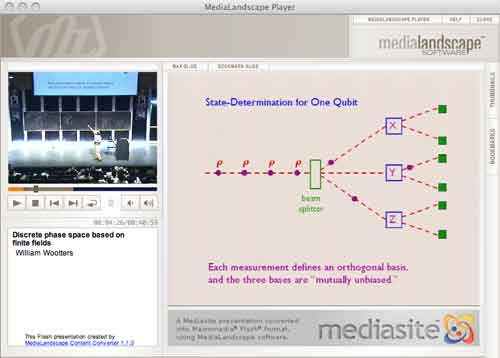
MUBs (for Mutually Unbiased Bases) are quite popular at the moment. Kea is running a mini-series Mutual Unbias as is Carl Brannen. Further, the Perimeter Institute has a good website for its seminars where they offer streaming video (I like their MacromediaFlash format giving video and slides/blackboard shots simultaneously, in distinct windows) including a talk on MUBs (as well as an old talk by Wootters).

So what are MUBs to mathematicians? Recall that a d-state quantum system is just the vectorspace $\mathbb{C}^d $ equipped with the usual Hermitian inproduct $\vec{v}.\vec{w} = \sum \overline{v_i} w_i $. An observable $E $ is a choice of orthonormal basis ${ \vec{e_i} } $ consisting of eigenvectors of the self-adjoint matrix $E $. $E $ together with another observable $F $ (with orthonormal basis ${ \vec{f_j} } $) are said to be mutally unbiased if the norms of all inproducts $\vec{f_j}.\vec{e_i} $ are equal to $1/\sqrt{d} $. This definition extends to a collection of pairwise mutually unbiased observables. In a d-state quantum system there can be at most d+1 mutually unbiased bases and such a collection of observables is then called a MUB of the system. Using properties of finite fields one has shown that MUBs exists whenever d is a prime-power. On the other hand, existence of a MUB for d=6 still seems to be open…

The King’s Problem (( actually a misnomer, it’s more the poor physicists’ problem… )) is the following : A physicist is trapped on an island ruled by a mean
king who promises to set her free if she can give him the answer to the following puzzle. The
physicist is asked to prepare a d−state quantum system in any state of her choosing and give it
to the king, who measures one of several mutually unbiased observables on it. Following this, the physicist is allowed to make a control measurement
on the system, as well as any other systems it may have been coupled to in the preparation
phase. The king then reveals which observable he measured and the physicist is required
to predict correctly all the eigenvalues he found.

The Solution to the King’s problem in prime power dimension by P. K. Aravind, say for $d=p^k $, consists in taking a system of k object qupits (when $p=2l+1 $ one qupit is a spin l particle) which she will give to the King together with k ancilla qupits that she retains in her possession. These 2k qupits are diligently entangled and prepared is a well chosen state. The final step in finding a suitable state is the solution to a pure combinatorial problem :

She must use the numbers 1 to d to form $d^2 $ ordered sets of d+1 numbers each, with repetitions of numbers within a set allowed, such that any two sets have exactly one identical number in the same place in both. Here’s an example of 16 such strings for d=4 :

11432, 12341, 13214, 14123, 21324, 22413, 23142, 24231, 31243, 32134, 33421, 34312, 41111, 42222, 43333, 44444

Here again, finite fields are used in the solution. When $d=p^k $, identify the elements of $\mathbb{F}_{p^k} $ with the numbers from 1 to d in some fixed way. Then, the $d^2 $ of number-strings are found as follows : let $k_0,k_1 \in \mathbb{F}_{p^k} $ and take as the first 2 numbers the ones corresponding to these field-elements. The remaning d-2 numbers in the string are those corresponding to the field element $k_m $ (with $2 \leq m \leq d $) determined from $k_0,k_1 $ by the equation

$k_m = l_{m} * k_0+k_1 $

where $l_i $ is the field-element corresponding to the integer i ($l_1 $ corresponds to the zero element). It is easy to see that these $d^2 $ strings satisfy the conditions of the combinatorial problem. Indeed, any two of its digits determine $k_0,k_1 $ (and hence the whole string) as it follows from
$k_m = l_m k_0 + k_1 $ and $k_r = l_r k_0 + k_1 $ that $k_0 = \frac{k_m-k_r}{l_m-l_r} $.

In the special case when d=3 (that is, one spin 1 particle is given to the King), we recover the tetracode : the nine codewords

0000, 0+++, 0—, +0+-, ++-0, +-0+, -0-+, -+0-, –+0

encode the strings (with +=1,-=2,0=3)

3333, 3111, 3222, 1312, 1123, 1231, 2321, 2132, 2213

Leave a Comment

KMS, Gibbs & zeta function

Time to wrap up this series on the Bost-Connes algebra. Here’s what we have learned so far : the convolution product on double cosets

$\begin{bmatrix} 1 & \mathbb{Z} \\ 0 & 1 \end{bmatrix} \backslash \begin{bmatrix} 1 & \mathbb{Q} \\ 0 & \mathbb{Q}_{> 0} \end{bmatrix} / \begin{bmatrix} 1 & \mathbb{Z} \\ 0 & 1 \end{bmatrix} $

is a noncommutative algebra, the Bost-Connes Hecke algebra $\mathcal{H} $, which is a bi-chrystalline graded algebra (somewhat weaker than ‘strongly graded’) with part of degree one the group-algebra $\mathbb{Q}[\mathbb{Q}/\mathbb{Z}] $. Further, $\mathcal{H} $ has a natural one-parameter family of algebra automorphisms $\sigma_t $ defined by $\sigma_t(X_n) = n^{it}X_n $ and $\sigma_t(Y_{\lambda})=Y_{\lambda} $.

For any algebra $A $ together with a one-parameter family of automorphisms $\sigma_t $ one is interested in KMS-states or Kubo-Martin-Schwinger states with parameter $\beta $, $KMS_{\beta} $ (this parameter is often called the ‘invers temperature’ of the system) as these are suitable equilibria states. Recall that a state is a special linear functional $\phi $ on $A $ (in particular it must have norm one) and it belongs to $KMS_{\beta} $ if the following commutation relation holds for all elements $a,b \in A $

$\phi(a \sigma_{i\beta}(b)) = \phi(b a) $

Let us work out the special case when $A $ is the matrix-algebra $M_n(\mathbb{C}) $. To begin, all algebra-automorphisms are inner in this case, so any one-parameter family of automorphisms is of the form

$\sigma_t(a) = e^{itH} a e^{-itH} $

where $e^{itH} $ is the matrix-exponential of the nxn matrix $H $. For any parameter $\beta $ we claim that the linear functional

$\phi(a) = \frac{1}{tr(e^{-\beta H})} tr(a e^{-\beta H}) $

is a KMS-state.Indeed, we have for all matrices $a,b \in M_n(\mathbb{C}) $ that

$\phi(a \sigma_{i \beta}(b)) = \frac{1}{tr(e^{-\beta H})} tr(a e^{- \beta H} b e^{\beta H} e^{- \beta H}) $

$= \frac{1}{tr(e^{-\beta H})} tr(a e^{-\beta H} b) = \frac{1}{tr(e^{-\beta H})} tr(ba e^{-\beta H}) = \phi(ba) $

(the next to last equality follows from cyclic-invariance of the trace map).
These states are usually called Gibbs states and the normalization factor $\frac{1}{tr(e^{-\beta H})} $ (needed because a state must have norm one) is called the partition function of the system. Gibbs states have arisen from the study of ideal gases and the place to read up on all of this are the first two chapters of the second volume of “Operator algebras and quantum statistical mechanics” by Ola Bratelli and Derek Robinson.

This gives us a method to construct KMS-states for an arbitrary algebra $A $ with one-parameter automorphisms $\sigma_t $ : take a simple n-dimensional representation $\pi~:~A \mapsto M_n(\mathbb{C}) $, find the matrix $H $ determining the image of the automorphisms $\pi(\sigma_t) $ and take the Gibbs states as defined before.

Let us return now to the Bost-Connes algebra $\mathcal{H} $. We don’t know any finite dimensional simple representations of $\mathcal{H} $ but, sure enough, have plenty of graded simple representations. By the usual strongly-graded-yoga they should correspond to simple finite dimensional representations of the part of degree one $\mathbb{Q}[\mathbb{Q}/\mathbb{Z}] $ (all of them being one-dimensional and corresponding to characters of $\mathbb{Q}/\mathbb{Z} $).

Hence, for any $u \in \mathcal{G} = \prod_p \hat{\mathbb{Z}}_p^{\ast} $ (details) we have a graded simple $\mathcal{H} $-representation $S_u = \oplus_{n \in \mathbb{N}_+} \mathbb{C} e_n $ with action defined by

$\begin{cases} \pi_u(X_n)(e_m) = e_{nm} \\ \pi_u(Y_{\lambda})(e_m) = e^{2\pi i n u . \lambda} e_m \end{cases} $

Here, $u.\lambda $ is computed using the ‘chinese-remainder-identification’ $\mathcal{A}/\mathcal{R} = \mathbb{Q}/\mathbb{Z} $ (details).

Even when the representations $S_u $ are not finite dimensional, we can mimic the above strategy : we should find a linear operator $H $ determining the images of the automorphisms $\pi_u(\sigma_t) $. We claim that the operator is defined by $H(e_n) = log(n) e_n $ for all $n \in \mathbb{N}_+ $. That is, we claim that for elements $a \in \mathcal{H} $ we have

$\pi_u(\sigma_t(a)) = e^{itH} \pi_u(a) e^{-itH} $

So let us compute the action of both sides on $e_m $ when $a=X_n $. The left hand side gives $\pi_u(n^{it}X_n)(e_m) = n^{it} e_{mn} $ whereas the right-hand side becomes

$e^{itH}\pi_u(X_n) e^{-itH}(e_m) = e^{itH} \pi_u(X_n) m^{-it} e_m = $

$e^{itH} m^{-it} e_{mn} = (mn)^{it} m^{-it} e_{mn} = n^{it} e_{mn} $

proving the claim. For any parameter $\beta $ this then gives us a KMS-state for the Bost-Connes algebra by

$\phi_u(a) = \frac{1}{Tr(e^{-\beta H})} Tr(\pi_u(a) e^{-\beta H}) $

Finally, let us calculate the normalization factor (or partition function) $\frac{1}{Tr(e^{-\beta H})} $. Because $e^{-\beta H}(e_n) = n^{-\beta} e_n $ we have for that the trace

$Tr(e^{-\beta H}) = \sum_{n \in \mathbb{N}_+} \frac{1}{n^{\beta}} = \zeta(\beta) $

is equal to the Riemann zeta-value $\zeta(\beta) $ (at least when $\beta > 1 $).

Summarizing, we started with the definition of the Bost-Connes algebra $\mathcal{H} $, found a canonical one-parameter subgroup of algebra automorphisms $\sigma_t $ and computed that the natural equilibria states with respect to this ‘time evolution’ have as their partition function the Riemann zeta-function. Voila!

Leave a Comment

“God given time”

If you ever sat through a lecture by Alain Connes you will know about his insistence on the ‘canonical dynamic nature of noncommutative manifolds’. If you haven’t, he did write a blog post Heart bit 1 about it.

I’ll try to explain here that there is a definite “supplément d’âme” obtained in the transition from classical (commutative) spaces to the noncommutative ones. The main new feature is that “noncommutative spaces generate their own time” and moreover can undergo thermodynamical operations such as cooling, distillation etc…

Here a section from his paper A view of mathematics :

Indeed even at the coarsest level of understanding of a space provided by measure
theory, which in essence only cares about the “quantity of points” in a space, one
finds unexpected completely new features in the noncommutative case. While it
had been long known by operator algebraists that the theory of von-Neumann
algebras represents a far reaching extension of measure theory, the main surprise
which occurred at the beginning of the seventies is that such an algebra M
inherits from its noncommutativity a god-given time evolution:

$\delta~:~\mathbb{R} \rightarrow Out(M) $

where $Out M = Aut M/Int M $ is the quotient of the group of automorphisms of M
by the normal subgroup of inner automorphisms. This led in my thesis to the
reduction from type III to type II and their automorphisms and eventually to the
classification of injective factors.

Even a commutative manifold has a kind of dynamics associated to it. Take a suitable vectorfield, consider the flow determined by it and there’s your ‘dynamics’, or a one-parameter group of automorphisms on the functions. Further, other classes of noncommutative algebras have similar features. For example, Cuntz and Quillen showed that also formally smooth algebras (the noncommutative manifolds in the algebraic world) have natural Yang-Mills flows associated to them, giving a one-parameter subgroup of automorphisms.

Let us try to keep far from mysticism and let us agree that by ‘time’ (let alone ‘god given time’) we mean a one-parameter subgroup of algebra automorphisms of the noncommutative algebra. In nice cases, such as some von-Neumann algebras this canonical subgroup is canonical in the sense that it is unique upto inner automorphisms.

In the special case of the Bost-Connes algebra these automorphisms $\sigma_t $ are given by $\sigma_t(X_n) = n^{it} X_n $ and $\sigma_t(Y_{\lambda}) = Y_{\lambda} $.

This one-parameter subgroup is crucial in the definition of the so called KMS-states (for Kubo-Martin and Schwinger) which is our next goal.

Leave a Comment