Category: featured

On2 : Conway’s nim-arithmetics

Published January 26, 2009 by lieven

Last time we did recall Cantor’s addition and multiplication on ordinal numbers. Note that we can identify an ordinal number $\alpha $ with (the order type of) the set of all strictly smaller ordinals, that is, $\alpha = { \alpha’~:~\alpha’ < \alpha } $. Given two ordinals $\alpha $ and $\beta $ we will denote their Cantor-sums and products as $[ \alpha + \beta] $ and $[\alpha . \beta] $.

The reason for these square brackets is that John Conway constructed a well behaved nim-addition and nim-multiplication on all ordinals $\mathbf{On}_2 $ by imposing the ‘simplest’ rules which make $\mathbf{On}_2 $ into a field. By this we mean that, in order to define the addition $\alpha + \beta $ we must have constructed before all sums $\alpha’ + \beta $ and $\alpha + \beta’ $ with $\alpha’ < \alpha $ and $\beta’ < \beta $. If + is going to be a well-defined addition on $\mathbf{On}_2 $ clearly $\alpha + \beta $ cannot be equal to one of these previously constructed sums and the ‘simplicity rule’ asserts that we should take $\alpha+\beta $ the least ordinal different from all these sums $\alpha’+\beta $ and $\alpha+\beta’ $. In symbols, we define

$\alpha+ \beta = \mathbf{mex} { \alpha’+\beta,\alpha+ \beta’~|~\alpha’ < \alpha, \beta’ < \beta } $

where $\mathbf{mex} $ stands for ‘minimal excluded value’. If you’d ever played the game of Nim you will recognize this as the Nim-addition, at least when $\alpha $ and $\beta $ are finite ordinals (that is, natural numbers) (to nim-add two numbers n and m write them out in binary digits and add without carrying). Alternatively, the nim-sum n+m can be found applying the following two rules :

the nim-sum of a number of distinct 2-powers is their ordinary sum (e.g. $8+4+1=13 $, and,
the nim-sum of two equal numbers is 0.

So, all we have to do is to write numbers n and m as sums of two powers, scratch equal terms and add normally. For example, $13+7=(8+4+1)+(4+2+1)=8+2=10 $ (of course this is just digital sum without carry in disguise).

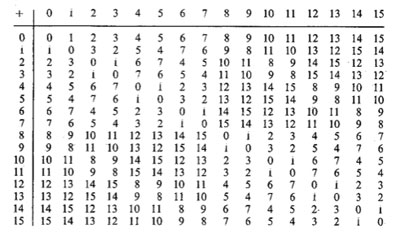
Here’s the beginning of the nim-addition table on ordinals. For example, to define $13+7 $ we have to look at all values in the first 7 entries of the row of 13 (that is, ${ 13,12,15,14,9,8,11 } $) and the first 13 entries in the column of 7 (that is, ${ 7,6,5,4,3,2,1,0,15,14,13,12,11 } $) and find the first number not included in these two sets (which is indeed $10 $).

In fact, the above two rules allow us to compute the nim-sum of any two ordinals. Recall from last time that every ordinal can be written uniquely as as a finite sum of (ordinal) 2-powers :
$\alpha = [2^{\alpha_0} + 2^{\alpha_1} + \ldots + 2^{\alpha_k}] $, so to determine the nim-sum $\alpha+\beta $ we write both ordinals as sums of ordinal 2-powers, delete powers appearing twice and take the Cantor ordinal sum of the remaining sum.

Nim-multiplication of ordinals is a bit more complicated. Here’s the definition as a minimal excluded value

$\alpha.\beta = \mathbf{mex} { \alpha’.\beta + \alpha.\beta’ – \alpha’.\beta’ } $

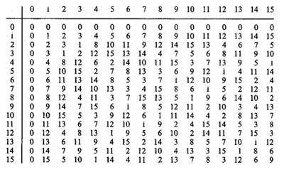
for all $\alpha’ < \alpha, \beta’ < \beta $. The rationale behind this being that both $\alpha-\alpha’ $ and $\beta – \beta’ $ are non-zero elements, so if $\mathbf{On}_2 $ is going to be a field under nim-multiplication, their product should be non-zero (and hence strictly greater than 0), that is, $~(\alpha-\alpha’).(\beta-\beta’) > 0 $. Rewriting this we get $\alpha.\beta > \alpha’.\beta+\alpha.\beta’-\alpha’.\beta’ $ and again the ‘simplicity rule’ asserts that $\alpha.\beta $ should be the least ordinal satisfying all these inequalities, leading to the $\mathbf{mex} $-definition above. The table gives the beginning of the nim-multiplication table for ordinals. For finite ordinals n and m there is a simple 2 line procedure to compute their nim-product, similar to the addition-rules mentioned before :

the nim-product of a number of distinct Fermat 2-powers (that is, numbers of the form $2^{2^n} $) is their ordinary product (for example, $16.4.2=128 $), and,
the square of a Fermat 2-power is its sesquimultiple (that is, the number obtained by multiplying with $1\frac{1}{2} $ in the ordinary sense). That is, $2^2=3,4^2=6,16^2=24,… $

Using these rules, associativity and distributivity and our addition rules it is now easy to work out the nim-multiplication $n.m $ : write out n and m as sums of (multiplications by 2-powers) of Fermat 2-powers and apply the rules. Here’s an example

$5.9=(4+1).(4.2+1)=4^2.2+4.2+4+1=6.2+8+4+1=(4+2).2+13=4.2+2^2+13=8+3+13=6 $

Clearly, we’d love to have a similar procedure to calculate the nim-product $\alpha.\beta $ of arbitrary ordinals, or at least those smaller than $\omega^{\omega^{\omega}} $ (recall that Conway proved that this ordinal is isomorphic to the algebraic closure $\overline{\mathbb{F}}_2 $ of the field of two elements). From now on we restrict to such ‘small’ ordinals and we introduce the following special elements :

$\kappa_{2^n} = [2^{2^{n-1}}] $ (these are the Fermat 2-powers) and for all primes $p > 2 $ we define
$\kappa_{p^n} = [\omega^{\omega^{k-1}.p^{n-1}}] $ where $k $ is the number of primes strictly smaller than $p $ (that is, for p=3 we have k=1, for p=5, k=2 etc.).

Again by associativity and distributivity we will be able to multiply two ordinals $< \omega^{\omega^{\omega}} $ if we know how to multiply a product

$[\omega^{\alpha}.2^{n_0}].[\omega^{\beta}.2^{m_0}] $ with $\alpha,\beta < [\omega^{\omega}] $ and $n_0,m_0 \in \mathbb{N} $.

Now, $\alpha $ can be written uniquely as $[\omega^t.n_t+\omega^{t-1}.n_{t-1}+\ldots+\omega.n_2 + n_1] $ with t and all $n_i $ natural numbers. Write each $n_k $ in base $p $ where $p $ is the $k+1 $-th prime number, that is, we have for $n_0,n_1,\ldots,n_t $ an expression

$n_k=[\sum_j p^j.m(j,k)] $ with $0 \leq m(j,k) < p $

The point of all this is that any of the special elements we want to multiply can be written as a unique expression as a decreasing product

$[\omega^{\alpha}.2^{n_0}] = [ \prod_q \kappa_q^m(q) ] $

where $q $ runs over all prime powers. The crucial fact now is that for this decreasing product we have a rule similar to addition of 2-powers, that is Conway-products coincide with the Cantor-products

$[ \prod_q \kappa_q^m(q) ] = \prod_q \kappa_q^m(q) $

But then, using associativity and commutativity of the Conway-product we can ‘nearly’ describe all products $[\omega^{\alpha}.2^{n_0}].[\omega^{\beta}.2^{m_0}] $. The remaining problem being that it may happen that for some q we will end up with an exponent $m(q)+m(q’)>p $. But this can be solved if we know how to take p-powers. The rules for this are as follows

$~(\kappa_{2^n})^2 = \kappa_{2^n} + \prod_{1 \leq i < n} \kappa_{2^i} $, for 2-powers, and,

$~(\kappa_{p^n})^p = \kappa_{p^{n-1}} $ for a prime $p > 2 $ and for $n \geq 2 $, and finally

$~(\kappa_p)^p = \alpha_p $ for a prime $p > 2 $, where $\alpha_p $ is the smallest ordinal $< \kappa_p $ which cannot be written as a p-power $\beta^p $ with $\beta < \kappa_p $. Summarizing : if we will be able to find these mysterious elements $\alpha_p $ for all prime numbers p, we are able to multiply in $[\omega^{\omega^{\omega}}]=\overline{\mathbb{F}}_2 $.

Let us determine the first one. We have that $\kappa_3 = \omega $ so we are looking for the smallest natural number $n < \omega $ which cannot be written in num-multiplication as $n=m^3 $ for $m < \omega $ (that is, also $m $ a natural number). Clearly $1=1^3 $ but what about 2? Can 2 be a third root of a natural number wrt. nim-multiplication? From the tabel above we see that 2 has order 3 whence its cube root must be an element of order 9. Now, the only finite ordinals that are subfields of $\mathbf{On}_2 $ are precisely the Fermat 2-powers, so if there is a finite cube root of 2, it must be contained in one of the finite fields $[2^{2^n}] $ (of which the mutiplicative group has order $2^{2^n}-1 $ and one easily shows that 9 cannot be a divisor of any of the numbers $2^{2^n}-1 $, that is, 2 doesn’t have a finte 3-th root in nim! Phrased differently, we found our first mystery number $\alpha_3 = 2 $. That is, we have the marvelous identity in nim-arithmetic

$\omega^3 = 2 $

Okay, so what is $\alpha_5 $? Well, we have $\kappa_5 = [\omega^{\omega}] $ and we have to look for the smallest ordinal which cannot be written as a 5-th root. By inspection of the finite nim-table we see that 1,2 and 3 have 5-th roots in $\omega $ but 4 does not! The reason being that 4 has order 15 (check in the finite field [16]) and 25 cannot divide any number of the form $2^{2^n}-1 $. That is, $\alpha_5=4 $ giving another crazy nim-identity

$~(\omega^{\omega})^5 = 4 $

And, surprises continue to pop up… Conway showed that $\alpha_7 = \omega+1 $ giving the nim-identity $~(\omega^{\omega^2})^7 = \omega+1 $. The proof of this already uses some clever finite field arguments. Because 7 doesn’t divide any number $2^{2^n}-1 $, none of the finite subfields $[2^{2^n}] $ contains a 7-th root of unity, so the 7-power map is injective whence surjective, so all finite ordinal have finite 7-th roots! That is, $\alpha_7 \geq \omega $. Because $\omega $ lies in a cubic extension of the finite field [4], the field generated by $\omega $ has 64 elements and so its multiplicative group is cyclic of order 63 and as $\omega $ has order 9, it must be a 7-th power in this field. But, as the only 7th powers in that field are precisely the powers of $\omega $ and by inspection $\omega+1 $ is not a 7-th power in that field (and hence also not in any field extension obtained by adjoining square, cube and fifth roots) so $\alpha_7=\omega +1 $.

Conway did stop at $\alpha_7 $ but I’ve always been intrigued by that one line in ONAG p.61 : “Hendrik Lenstra has computed $\alpha_p $ for $p \leq 43 $”. Next time we will see how Lenstra managed to do this and we will use sage to extend his list a bit further, including the first open case : $\alpha_{47}= \omega^{\omega^7}+1 $.

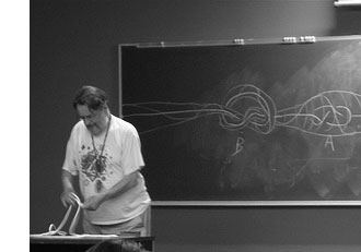
For an enjoyable video on all of this, see Conway’s MSRI lecture on Infinite Games. The nim-arithmetic part is towards the end of the lecture but watching the whole video is a genuine treat!

Comments closed

Mumford’s treasure map

Published December 13, 2008 by lieven

David Mumford did receive earlier this year the 2007 AMS Leroy P. Steele Prize for Mathematical Exposition. The jury honors Mumford for “his beautiful expository accounts of a host of aspects of algebraic geometry”. Not surprisingly, the first work they mention are his mimeographed notes of the first 3 chapters of a course in algebraic geometry, usually called “Mumford’s red book” because the notes were wrapped in a red cover. In 1988, the notes were reprinted by Springer-Verlag. Unfortnately, the only red they preserved was in the title.

The AMS describes the importance of the red book as follows. “This is one of the few books that attempt to convey in pictures some of the highly abstract notions that arise in the field of algebraic geometry. In his response upon receiving the prize, Mumford recalled that some of his drawings from The Red Book were included in a collection called Five Centuries of French Mathematics. This seemed fitting, he noted: “After all, it was the French who started impressionist painting and isn’t this just an impressionist scheme for rendering geometry?””

These days it is perfectly possible to get a good grasp on difficult concepts from algebraic geometry by reading blogs, watching YouTube or plugging in equations to sophisticated math-programs. In the early seventies though, if you wanted to know what Grothendieck’s scheme-revolution was all about you had no choice but to wade through the EGA’s and SGA’s and they were notorious for being extremely user-unfriendly regarding illustrations…

So the few depictions of schemes available, drawn by people sufficiently fluent in Grothendieck’s new geometric language had no less than treasure-map-cult-status and were studied in minute detail. Mumford’s red book was a gold mine for such treasure maps. Here’s my favorite one, scanned from the original mimeographed notes (it looks somewhat tidier in the Springer-version)

It is the first depiction of $\mathbf{spec}(\mathbb{Z}[x]) $, the affine scheme of the ring $\mathbb{Z}[x] $ of all integral polynomials. Mumford calls it the”arithmetic surface” as the picture resembles the one he made before of the affine scheme $\mathbf{spec}(\mathbb{C}[x,y]) $ corresponding to the two-dimensional complex affine space $\mathbb{A}^2_{\mathbb{C}} $. Mumford adds that the arithmetic surface is ‘the first example which has a real mixing of arithmetic and geometric properties’.

Let’s have a closer look at the treasure map. It introduces some new signs which must have looked exotic at the time, but have since become standard tools to depict algebraic schemes.

For starters, recall that the underlying topological space of $\mathbf{spec}(\mathbb{Z}[x]) $ is the set of all prime ideals of the integral polynomial ring $\mathbb{Z}[x] $, so the map tries to list them all as well as their inclusions/intersections.

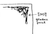
The doodle in the right upper corner depicts the ‘generic point’ of the scheme. That is, the geometric object corresponding to the prime ideal $~(0) $ (note that $\mathbb{Z}[x] $ is an integral domain). Because the zero ideal is contained in any other prime ideal, the algebraic/geometric mantra (“inclusions reverse when shifting between algebra and geometry”) asserts that the gemetric object corresponding to $~(0) $ should contain all other geometric objects of the arithmetic plane, so it is just the whole plane! Clearly, it is rather senseless to depict this fact by coloring the whole plane black as then we wouldn’t be able to see the finer objects. Mumford’s solution to this is to draw a hairy ball, which in this case, is sufficiently thick to include fragments going in every possible direction. In general, one should read these doodles as saying that the geometric object represented by this doodle contains all other objects seen elsewhere in the picture if the hairy-ball-doodle includes stuff pointing in the direction of the smaller object. So, in the case of the object corresponding to $~(0) $, the doodle has pointers going everywhere, saying that the geometric object contains all other objects depicted.

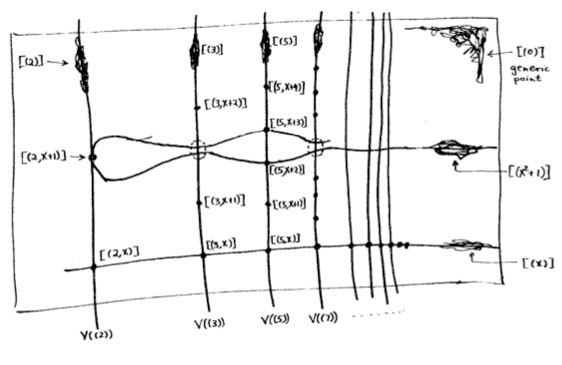
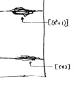
Let’s move over to the doodles in the lower right-hand corner. They represent the geometric object corresponding to principal prime ideals of the form $~(p(x)) $, where $p(x) $ in an irreducible polynomial over the integers, that is, a polynomial which we cannot write as the product of two smaller integral polynomials. The objects corresponding to such prime ideals should be thought of as ‘horizontal’ curves in the plane.

The doodles depicted correspond to the prime ideal $~(x) $, containing all polynomials divisible by $x $ so when we divide it out we get, as expected, a domain $\mathbb{Z}[x]/(x) \simeq \mathbb{Z} $, and the one corresponding to the ideal $~(x^2+1) $, containing all polynomials divisible by $x^2+1 $, which can be proved to be a prime ideals of $\mathbb{Z}[x] $ by observing that after factoring out we get $\mathbb{Z}[x]/(x^2+1) \simeq \mathbb{Z}[i] $, the domain of all Gaussian integers $\mathbb{Z}[i] $. The corresponding doodles (the ‘generic points’ of the curvy-objects) have a predominant horizontal component as they have the express the fact that they depict horizontal curves in the plane. It is no coincidence that the doodle of $~(x^2+1) $ is somewhat bulkier than the one of $~(x) $ as the later one must only depict the fact that all points lying on the straight line to its left belong to it, whereas the former one must claim inclusion of all points lying on the ‘quadric’ it determines.

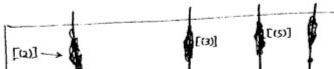
Apart from these ‘horizontal’ curves, there are also ‘vertical’ lines corresponding to the principal prime ideals $~(p) $, containing the polynomials, all of which coefficients are divisible by the prime number $p $. These are indeed prime ideals of $\mathbb{Z}[x] $, because their quotients are
$\mathbb{Z}[x]/(p) \simeq (\mathbb{Z}/p\mathbb{Z})[x] $ are domains, being the ring of polynomials over the finite field $\mathbb{Z}/p\mathbb{Z} = \mathbb{F}_p $. The doodles corresponding to these prime ideals have a predominant vertical component (depicting the ‘vertical’ lines) and have a uniform thickness for all prime numbers $p $ as each of them only has to claim ownership of the points lying on the vertical line under them.

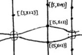
Right! So far we managed to depict the zero prime ideal (the whole plane) and the principal prime ideals of $\mathbb{Z}[x] $ (the horizontal curves and the vertical lines). Remains to depict the maximal ideals. These are all known to be of the form
$\mathfrak{m} = (p,f(x)) $
where $p $ is a prime number and $f(x) $ is an irreducible integral polynomial, which remains irreducible when reduced modulo $p $ (that is, if we reduce all coefficients of the integral polynomial $f(x) $ modulo $p $ we obtain an irreducible polynomial in $~\mathbb{F}_p[x] $). By the algebra/geometry mantra mentioned before, the geometric object corresponding to such a maximal ideal can be seen as the ‘intersection’ of an horizontal curve (the object corresponding to the principal prime ideal $~(f(x)) $) and a vertical line (corresponding to the prime ideal $~(p) $). Because maximal ideals do not contain any other prime ideals, there is no reason to have a doodle associated to $\mathfrak{m} $ and we can just depict it by a “point” in the plane, more precisely the intersection-point of the horizontal curve with the vertical line determined by $\mathfrak{m}=(p,f(x)) $. Still, Mumford’s treasure map doesn’t treat all “points” equally. For example, the point corresponding to the maximal ideal $\mathfrak{m}_1 = (3,x+2) $ is depicted by a solid dot $\mathbf{.} $, whereas the point corresponding to the maximal ideal $\mathfrak{m}_2 = (3,x^2+1) $ is represented by a fatter point $\circ $. The distinction between the two ‘points’ becomes evident when we look at the corresponding quotients (which we know have to be fields). We have

$\mathbb{Z}[x]/\mathfrak{m}_1 = \mathbb{Z}[x]/(3,x+2)=(\mathbb{Z}/3\mathbb{Z})[x]/(x+2) = \mathbb{Z}/3\mathbb{Z} = \mathbb{F}_3 $ whereas $\mathbb{Z}[x]/\mathfrak{m}_2 = \mathbb{Z}[x]/(3,x^2+1) = \mathbb{Z}/3\mathbb{Z}[x]/(x^2+1) = \mathbb{F}_3[x]/(x^2+1) = \mathbb{F}_{3^2} $

because the polynomial $x^2+1 $ remains irreducible over $\mathbb{F}_3 $, the quotient $\mathbb{F}_3[x]/(x^2+1) $ is no longer the prime-field $\mathbb{F}_3 $ but a quadratic field extension of it, that is, the finite field consisting of 9 elements $\mathbb{F}_{3^2} $. That is, we represent the ‘points’ lying on the vertical line corresponding to the principal prime ideal $~(p) $ by a solid dot . when their quotient (aka residue field is the prime field $~\mathbb{F}_p $, by a bigger point $\circ $ when its residue field is the finite field $~\mathbb{F}_{p^2} $, by an even fatter point $\bigcirc $ when its residue field is $~\mathbb{F}_{p^3} $ and so on, and on. The larger the residue field, the ‘fatter’ the corresponding point.

In fact, the ‘fat-point’ signs in Mumford’s treasure map are an attempt to depict the fact that an affine scheme contains a lot more information than just the set of all prime ideals. In fact, an affine scheme determines (and is determined by) a “functor of points”. That is, to every field (or even every commutative ring) the affine scheme assigns the set of its ‘points’ defined over that field (or ring). For example, the $~\mathbb{F}_p $-points of $\mathbf{spec}(\mathbb{Z}[x]) $ are the solid . points on the vertical line $~(p) $, the $~\mathbb{F}_{p^2} $-points of $\mathbf{spec}(\mathbb{Z}[x]) $ are the solid . points and the slightly bigger $\circ $ points on that vertical line, and so on.

This concludes our first attempt to decypher Mumford’s drawing, but if we delve a bit deeper, we are bound to find even more treasures… (to be continued).

Comments closed

Connes-Consani for undergraduates (3)

Published October 10, 2008 by lieven

A quick recap of last time. We are trying to make sense of affine varieties over the elusive field with one element $\mathbb{F}_1 $, which by Grothendieck’s scheme-philosophy should determine a functor

$\mathbf{nano}(N)~:~\mathbf{abelian} \rightarrow \mathbf{sets} \qquad A \mapsto N(A) $

from finite Abelian groups to sets, typically giving pretty small sets $N(A) $. Using the F_un mantra that $\mathbb{Z} $ should be an algebra over $\mathbb{F}_1 $ any $\mathbb{F}_1 $-variety determines an integral scheme by extension of scalars, as well as a complex variety (by extending further to $\mathbb{C} $). We have already connected the complex variety with the original functor into a gadget that is a couple $~(\mathbf{nano}(N),\mathbf{maxi}(R)) $ where $R $ is the coordinate ring of a complex affine variety $X_R $ having the property that every element of $N(A) $ can be realized as a $\mathbb{C} A $-point of $X_R $. Ringtheoretically this simply means that to every element $x \in N(A) $ there is an algebra map $N_x~:~R \rightarrow \mathbb{C} A $.

Today we will determine which gadgets determine an integral scheme, and do so uniquely, and call them the sought for affine schemes over $\mathbb{F}_1 $.

Let’s begin with our example : $\mathbf{nano}(N) = \underline{\mathbb{G}}_m $ being the forgetful functor, that is $N(A)=A $ for every finite Abelian group, then the complex algebra $R= \mathbb{C}[x,x^{-1}] $ partners up to form a gadget because to every element $a \in N(A)=A $ there is a natural algebra map $N_a~:~\mathbb{C}[x,x^{-1}] \rightarrow \mathbb{C} A $ defined by sending $x \mapsto e_a $. Clearly, there is an obvious integral form of this complex algebra, namely $\mathbb{Z}[x,x^{-1}] $ but we have already seen that this algebra represents the mini-functor

$\mathbf{min}(\mathbb{Z}[x,x^{-1}])~:~\mathbf{abelian} \rightarrow \mathbf{sets} \qquad A \mapsto (\mathbb{Z} A)^* $

and that the group of units $(\mathbb{Z} A)^* $ of the integral group ring $\mathbb{Z} A $ usually is a lot bigger than $N(A)=A $. So, perhaps there is another less obvious $\mathbb{Z} $-algebra $S $ doing a much better job at approximating $N $? That is, if we can formulate this more precisely…

In general, every $\mathbb{Z} $-algebra $S $ defines a gadget $\mathbf{gadget}(S) = (\mathbf{mini}(S),\mathbf{maxi}(S \otimes_{\mathbb{Z}} \mathbb{C})) $ with the obvious (that is, extension of scalars) evaluation map

$\mathbf{mini}(S)(A) = Hom_{\mathbb{Z}-alg}(S, \mathbb{Z} A) \rightarrow Hom_{\mathbb{C}-alg}(S \otimes_{\mathbb{Z}} \mathbb{C}, \mathbb{C} A) = \mathbf{maxi}(S \otimes_{\mathbb{Z}} \mathbb{C})(A) $

Right, so how might one express the fact that the integral affine scheme $X_T $ with integral algebra $T $ is the ‘best’ integral approximation of a gadget $~(\mathbf{nano}(N),\mathbf{maxi}(R)) $. Well, to begin its representing functor should at least contain the information given by $N $, that is, $\mathbf{nano}(N) $ is a sub-functor of $\mathbf{mini}(T) $ (meaning that for every finite Abelian group $A $ we have a natural inclusion $N(A) \subset Hom_{\mathbb{Z}-alg}(T, \mathbb{Z} A) $). As to the “best”-part, we must express that all other candidates factor through $T $. That is, suppose we have an integral algebra $S $ and a morphism of gadgets (as defined last time)

$f~:~(\mathbf{nano}(N),\mathbf{maxi}(R)) \rightarrow \mathbf{gadget}(S) = (\mathbf{mini}(S),\mathbf{maxi}(S \otimes_{\mathbb{Z}} \mathbb{C})) $

then there ought to be $\mathbb{Z} $-algebra morphism $T \rightarrow S $ such that the above map $f $ factors through an induced gadget-map $\mathbf{gadget}(T) \rightarrow \mathbf{gadget}(S) $.

Fine, but is this definition good enough in our trivial example? In other words, is the “obvious” integral ring $\mathbb{Z}[x,x^{-1}] $ the best integral choice for approximating the forgetful functor $N=\underline{\mathbb{G}}_m $? Well, take any finitely generated integral algebra $S $, then saying that there is a morphism of gadgets from $~(\underline{\mathbb{G}}_m,\mathbf{maxi}(\mathbb{C}[x,x^{-1}]) $ to $\mathbf{gadget}(S) $ means that there is a $\mathbb{C} $-algebra map $\psi~:~S \otimes_{\mathbb{Z}} \mathbb{C} \rightarrow \mathbb{C}[x,x^{-1}] $ such that for every finite Abelian group $A $ we have a commuting diagram

$\xymatrix{A \ar[rr] \ar[d]_e & & Hom_{\mathbb{Z}-alg}(S, \mathbb{Z} A) \ar[d] \\
Hom_{\mathbb{C}-alg}(\mathbb{C}[x,x^{-1}],\mathbb{C} A) \ar[rr]^{- \circ \psi} & & Hom_{\mathbb{C}-alg}(S \otimes_{\mathbb{Z}} \mathbb{C}, \mathbb{C} A)} $

Here, $e $ is the natural evaluation map defined before sending a group-element $a \in A $ to the algebra map defined by $x \mapsto e_a $ and the vertical map on the right-hand side is extensions by scalars. From this data we must be able to show that the image of the algebra map

$\xymatrix{S \ar[r]^{i} & S \otimes_{\mathbb{Z}} \mathbb{C} \ar[r]^{\psi} & \mathbb{C}[x,x^{-1}]} $

is contained in the integral subalgebra $\mathbb{Z}[x,x^{-1}] $. So, take any generator $z $ of $S $ then its image $\psi(z) \in \mathbb{C}[x,x^{-1}] $ is a Laurent polynomial of degree say $d $ (that is, $\psi(z) = c_{-d} x^{-d} + \ldots c_{-1} x^{-1} + c_0 + c_1 x + \ldots + c_d x^d $ with all coefficients a priori in $\mathbb{C} $ and we need to talk them into $\mathbb{Z} $).

Now comes the basic trick : take a cyclic group $A=C_N $ of order $N > d $, then the above commuting diagram applied to the generator of $C_N $ (the evaluation of which is the natural projection map $\pi~:~\mathbb{C}[x.x^{-1}] \rightarrow \mathbb{C}[x,x^{-1}]/(x^N-1) = \mathbb{C} C_N $) gives us the commuting diagram

$\xymatrix{S \ar[r] \ar[d] & S \otimes_{\mathbb{Z}} \mathbb{C} \ar[r]^{\psi} & \mathbb{C}[x,x^{-1}] \ar[d]^{\pi} \\
\mathbb{Z} C_n = \frac{\mathbb{Z}[x,x^{-1}]}{(x^N-1)} \ar[rr]^j & & \frac{\mathbb{C}[x,x^{-1}]}{(x^N-1)}} $

where the horizontal map $j $ is the natural inclusion map. Tracing $z \in S $ along the diagram we see that indeed all coefficients of $\psi(z) $ have to be integers! Applying the same argument to the other generators of $S $ (possibly for varying values of N) we see that , indeed, $\psi(S) \subset \mathbb{Z}[x,x^{-1}] $ and hence that $\mathbb{Z}[x,x^{-1}] $ is the best integral approximation for $\underline{\mathbb{G}}_m $.

That is, we have our first example of an affine variety over the field with one element $\mathbb{F}_1 $ : $~(\underline{\mathbb{G}}_m,\mathbf{maxi}(\mathbb{C}[x,x^{-1}]) \rightarrow \mathbf{gadget}(\mathbb{Z}[x,x^{-1}]) $.

What makes this example work is that the infinite group $\mathbb{Z} $ (of which the complex group-algebra is the algebra $\mathbb{C}[x,x^{-1}] $) has enough finite Abelian group-quotients. In other words, $\mathbb{F}_1 $ doesn’t see $\mathbb{Z} $ but rather its profinite completion $\hat{\mathbb{Z}} = \underset{\leftarrow} \mathbb{Z}/N\mathbb{Z} $… (to be continued when we’ll consider noncommutative $\mathbb{F}_1 $-schemes)

In general, an affine $\mathbb{F}_1 $-scheme is a gadget with morphism of gadgets
$~(\mathbf{nano}(N),\mathbf{maxi}(R)) \rightarrow \mathbf{gadget}(S) $ provided that the integral algebra $S $ is the best integral approximation in the sense made explicit before. This rounds up our first attempt to understand the Connes-Consani approach to define geometry over $\mathbb{F}_1 $ apart from one important omission : we have only considered functors to $\mathbf{sets} $, whereas it is crucial in the Connes-Consani paper to consider more generally functors to graded sets. In the final part of this series we’ll explain what that’s all about.