Skip to content →

Category: featured

Monsieur Mathieu

Even a virtual course needs an opening line, so here it is : Take your favourite $SL_2(\mathbb{Z}) $-representation Here is mine : the permutation presentation of the Mathieu group(s). Emile Leonard Mathieu is remembered especially for his discovery (in 1861 and 1873) of five sporadic simple groups named after him, the Mathieu groups $M_{11},M_{12},M_{22},M_{23} $ and $M_{24} $. These were studied in his thesis on transitive functions. He had a refreshingly direct style
of writing. I’m not sure what Cauchy would have thought (Cauchy died in 1857) about this ‘acknowledgement’ in his 1861-paper in which Mathieu describes $M_{12} $ and claims the construction of $M_{24} $.

Also the opening sentenses of his 1873 paper are nice, something along the lines of “if no expert was able to fill in the details of my claims made twelve years ago, I’d better do it myself”.

However, even after this paper opinions remained divided on the issue whether or not he did really achieve his goal, and the matter was settled decisively by Ernst Witt connecting the Mathieu groups to Steiner systems (if I recall well from Mark Ronan’s book Symmetry and the monster)

As Mathieu observed, the quickest way to describe these groups would be to give generators, but as these groups are generated by two permutations on 12 respectively 24 elements, we need to have a mnemotechnic approach to be able to reconstruct them whenever needed.

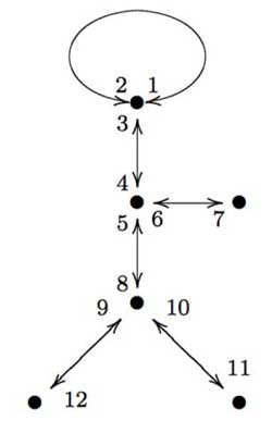
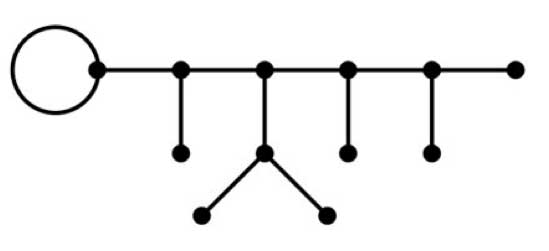
Here is a nice approach, due to Gunther Malle in a Luminy talk in 1993 on “Dessins d’enfants” (more about them later). Consider the drawing of “Monsieur Mathieu” on the left. That is, draw the left-handed bandit picture on 6 edges and vertices, divide each edge into two and give numbers to both parts (the actual numbering is up to you, but for definiteness let us choose the one on the left). Then, $M_{12} $ is generated by the order two permutation describing the labeling of both parts of the edges

$s=(1,2)(3,4)(5,8)(7,6)(9,12)(11,10) $

together with the order three permutation obtained from cycling counterclockwise
around a trivalent vertex and calling out the labels one encounters. For example, the three cycle corresponding to the ‘neck vertex’ is $~(1,2,3) $ and the total permutation
is

$t=(1,2,3)(4,5,6)(8,9,10) $

A quick verification using GAP tells that these elements do indeed generate a simple group of order 95040.

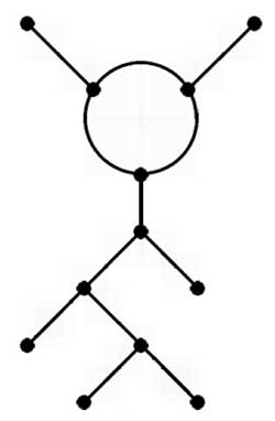
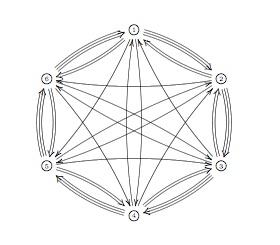
Similarly, if you have to reconstruct the largest Mathieu group from scratch, apply the same method to the the picture above or to “ET Mathieu” drawing on the left. This picture I copied from Alexander Zvonkin‘s paper How to draw a group as well as the computational details below.

This is all very nice and well but what do these drawings have to do with Grothendieck’s “dessins d’enfants”? Consider the map from the projective line onto itself

$\mathbb{P}^1_{\mathbb{C}} \rightarrow \mathbb{P}^1_{\mathbb{C}}$

defined by the rational map

$f(z) = \frac{(z^3-z^2+az+b)^3(z^3+cz^2+dz+e)}{Kz} $

where N. Magot calculated that

$a=\frac{107+7 \sqrt{-11}}{486},
b=-\frac{13}{567}a+\frac{5}{1701}, c=-\frac{17}{9},
d=\frac{23}{7}a+\frac{256}{567},
e=-\frac{1573}{567}a+\frac{605}{1701} $

and finally

$K =
-\frac{16192}{301327047}a+\frac{10880}{903981141} $

One verifies that this map is 12 to 1 everywhere except over the points ${
0,1,\infty } $ (that is, there are precisely 12 points mapping under f to a given point of $\mathbb{P}^1_{\mathbb{C}} – { 0,1,\infty } $. From the expression of f(z) it is clear that over 0 there lie 6 points (3 of which with multiplicity three, the others of multiplicity one). Over $\infty $ there are two points, one with multiplicity 11 and one with multiplicity one. The difficult part is to compute the points lying over 1. The miraculous fact of the given values is that

$f(z)-1 = \frac{-B(z)^2}{Kz} $

where

$B(z)=z^6+\frac{1}{11}(10c-8)z^5+(5a+9d-7c)z^4+(2b+4ac+8e-6d)z^3+$
$(3ad+bc-5e)z^2+2aez-be) $

and hence there are 6 points lying over 1 each with mutiplicity two.

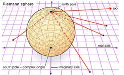
Right, now consider the complex projective line $\mathbb{P}^1_{\mathbb{C}} $ as the Riemann sphere $S^2 $ and mark the six points lying over 1 by a white vertex and the six points lying over 0 with a black vertex (in the source sphere). Now, lift the real interval $[0,1] $ in the target sphere $\mathbb{P}^1_{\mathbb{C}} = S^2 $ to its inverse image on the source sphere. As there are exactly 12 points lying over each real
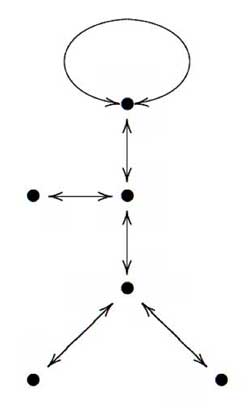
number $0 \lneq r \lneq 1 $, this inverse image will consist of 12 edges which are noncrossing and each end in one black and one white vertex. The obtained graph will look like the \”Monsieur Mathieu\” drawing above with the vertices corresponding to the black vertices and the three points over 1 of multiplicity three corresponding to the
trivalent vertices, those of multiplicity one to the three end-vertices. The white vertices correspond to mid-points of the six edges, so that we do get a drawing with twelve edges, one corresponding to each number. From the explicit description of f(z) it is clear that this map is defined over $\mathbb{Q}\sqrt{-11} $ which is also the
smallest field containing all character-values of the Mathieu group $M_{12} $. Further, the Galois group of the extension $Gal(\mathbb{Q}\sqrt{-11}/\mathbb{Q}) =
\mathbb{Z}/2\mathbb{Z} $ and is generated by complex conjugation. So, one might wonder what would happen if we replaced in the definition of the rational map f(z) the value of a by $a = \frac{107-\sqrt{-11}}{486} $. It turns out that this modified map has the same properties as $f(z) $ so again one can draw on the source sphere a picture consisting of twelve edges each ending in a white and black vertex.

If we consider the white vertices (which incidentally each lie on two edges as all points lying over 0 are of multiplicity two) as mid-points of longer edges connecting the
black vertices we obtain a drawing on the sphere which looks like \”Monsieur Mathieu\” but this time as a right handed bandit, and applying our mnemotechnic rule we obtain _another_ (non conjugated) embedding of $M_{12} $ in the full symmetric group on 12 vertices.

What is the connection with $SL_2(\mathbb{Z}) $-representations? Well, the permutation generators s and t of $M_{12} $ (or $M_{24} $ for that matter) have orders two and three, whence there is a projection from the free group product $C_2 \star C_3 $ (here $C_n $ is just the cyclic group of order n) onto $M_{12} $ (respectively $M_{24} $). Next
time we will say more about such free group products and show (among other things) that $PSL_2(\mathbb{Z}) \simeq C_2 \star C_3 $ whence the connection with $SL_2(\mathbb{Z}) $. In a following lecture we will extend the Monsieur Mathieu example to
arbitrary dessins d\’enfants which will allow us to assign to curves defined over $\overline{\mathbb{Q}} $ permutation representations of $SL_2(\mathbb{Z}) $ and other _cartographic groups_ such as the congruence subgroups $\Gamma_0(2) $ and
$\Gamma(2) $.

Leave a Comment

coalgebras and non-geometry 3

Last
time we saw that the _coalgebra of distributions_ of a
noncommutative manifold can be described as a coalgebra
Takeuchi-equivalent to the path coalgebra of a huge quiver. This
infinite quiver has as its vertices the isomorphism classes of finite
dimensional simple representations of the qurve A (the coordinate ring
of the noncommutative manifold) and there are as many directed arrows
between the vertices corresponding to the simples S and T as is the
dimension of $Ext^1_A(S,T) $.

The fact that this
coalgebra of distributions is equivalent to the path coalgebra of
_some_ quiver is in the Kontsevich-Soibelman
paper
though it would have been nice if they had given reference for
this fact to the paper Wedge Products and
Cotensor Coalgebras in Monoidal Categories
by Ardizzoni or to
previous work by P. Jara, D. Llena, L. Merino and D. Stefan,
“Hereditary and formally smooth coalgebras”, Algebr.
Represent. Theory 8 (2005), 363-374. In those papers it is shown that a
coalgebra with coseparable coradical is hereditary if and only if it
is formally smooth if and only if it is a cotensor coalgebra of some
bicomodule.

At first this looks just like the dual version of
the classical result that a finite dimensional hereditary algebra is
Morita equivalent to the path algebra of a quiver (which is indeed what
the proof does) but again the condition that the coradical is
coseparable does not require the coradical to be finite dimensional…
In our case, the coradical is indeed coseparable being the direct sum
over all matrix coalgebras corresponding to the simple representations.
Hence, we can again recover the _points_ of our noncommutative manifold
from the direct summands of the coradical. Fortunately, one can
compute this huge coalgebra of distributions from a small quiver, the
_one quiver to rule them all_, but as I’ve been babbling about all of
this here [numerous
times](https://lievenlb.local/?s=one+quiver) I’ll let the
interested find out for themselves how you use it (a) to get at the
isoclasses of all simples (hint : morally they are the smooth points of
the quotient varieties of n-dimensional representations and enough tools
have been developed recently to spot some fake simples, that is smooth
proper semi-simple points) and (b) to compute the _ragball_, that is the
huge quiver with vertex set the simples and arows as described
above. Over the years I’ve calculated several one-quivers for a
variety of qurves (such as amalgamated free products of finite groups
and smooth curves). If you are in for a puzzle, try to determine it for
the qurve $~(\mathbb{C}[x] \ast C_2) \ast_{\mathbb{C}
C_2} \mathbb{C} PSL_2(\mathbb{Z}) \ast_{\mathbb{C} C_3}
(\mathbb{C}[x] \ast C_3) $ The answer is a mysterious
hexagon

Leave a Comment

coalgebras and non-geometry 2

Last time we
have seen that the _coalgebra of distributions_ of an affine smooth
variety is the direct sum (over all points) of the dual to the etale
local algebras which are all of the form $\mathbb{C}[[
x_1,\ldots,x_d ]] $ where $d $ is the dimension of the
variety. Generalizing this to _non-commutative_ manifolds, the first
questions are : “What is the analogon of the power-series algebra?” and
do all ‘points’ of our non-commutative manifold do have such local
algebras? Surely, we no longer expect the variables to commute, so a
non-commutative version of the power series algebra should be
$\mathbb{C} \langle \langle x_1,\ldots,x_d \rangle \rangle $,
the ring of formal power series in non-commuting variables. However,
there is still another way to add non-commutativity and that is to go
from an algebra to matrices over the algebra. So, in all we would expect
to be our _local algebras_ at points of our non-commutative manifold to
be isomorphic to $M_n(\mathbb{C} \langle \langle x_1,\ldots,x_d
\rangle \rangle) $ As to the second question : _qurves_ (that is,
the coordinate rings of non-commutative manifolds) do have such algebras
as local rings provided we take as the ‘points’ of the non-commutative
variety the set of all _simple_ finite dimensional representations of
the qurve. This is a consequence of the _tubular neighborhood theorem_
due to [Cuntz](http://wwwmath.uni-muenster.de/u/cuntz/cuntz.html) and
[Quillen](http://www-history.mcs.st-andrews.ac.uk/Mathematicians/Quillen.html). In more details : If A is a qurve, then a simple
$n $-dimensional representation corresponds to an epimorphism
$\pi~:~A \rightarrow S = M_n(\mathbb{C}) $ and if we take
$\mathfrak{m}=Ker(\pi) $, then
$M=\mathfrak{m}/\mathfrak{m}^2 $ is an $S $-bimodule and
the $\mathfrak{m} $-adic completion of A is isomorphic to the
completed tensor-algebra $\hat{T}_S(M) \simeq M_n(\mathbb{C}
\langle \langle x_1,\ldots,x_d \rangle \rangle) $ In contrast with
the commutative case however where the dimension remains constant over
all points, here the numbers n and d can change from simple to simple.
For n this is clear as it gives the dimension of the simple
representation, but also d changes (it is the local dimension of the
variety classifying simple representations of the same dimension). Here
an easy example : Consider the skew group algebra $A =
\mathbb{C}[x] \star C_2 $ with the action given by sending $x
\mapsto -x $. Then A is a qurve and its center is
$\mathbb{C}[y] $ with $y=x^2 $. Over any point $y
\not= 0 $ there is a unique simple 2-dimensional representation of A
giving the local algebra $M_2(\mathbb{C}[[y]]) $. If
$y=0 $ the situation is more complicated as the local structure
of A is given by the algebra $\begin{bmatrix} \mathbb{C}[[y]] &
\mathbb{C}[[y]] \\ (y) & \mathbb{C}[[y]] \end{bmatrix} $ So, over
this point there are precisely 2 one-dimensional simple representations
corresponding to the maximal ideals $\mathfrak{m}_1 =
\begin{bmatrix} (y) & \mathbb{C}[[y]] \\ (y) & \mathbb{C}[[y]]
\end{bmatrix}~\qquad \text{and}~\qquad \mathfrak{m}_2 = \begin{bmatrix}
\mathbb{C}[[y]] & \mathbb{C}[[y]] \\ (y) & (y) \end{bmatrix} $ and
both ideals are idempotent, that is $\mathfrak{m}_i^2 =
\mathfrak{m}_i $ whence the corresponding bimodule $M_i =
0 $ so the local algebra in either of these two points is just
$\mathbb{C} $. Ok, so the comleted local algebra at each point
is of the form $M_n(\mathbb{C}\langle \langle x_1,\ldots,x_d \rangle
\rangle) $, but what is the corresponding dual coalgebra. Well,
$\mathbb{C} \langle \langle x_1,\ldots,x_d \rangle \rangle $ is
the algebra dual to the _cofree coalgebra_ on $V = \mathbb{C} x_1 +
\ldots + \mathbb{C}x_d $. As a vectorspace this is the
tensor-algebra $T(V) = \mathbb{C} \langle x_1,\ldots,x_d
\rangle $ with the coalgebra structure induced by the bialgebra
structure defined by taking all varaibales to be primitives, that is
$\Delta(x_i) = x_i \otimes 1 + 1 \otimes x_i $. That is, the
coproduct on a monomial gives all different expressions $m_1 \otimes
m_2 $ such that $m_1m_2 = m $. For example,
$\Delta(x_1x_2) = x_1x_2 \otimes 1 + x_1 \otimes x_2 + 1 \otimes
x_1x_2 $. On the other hand, the dual coalgebra of
$M_n(\mathbb{C}) $ is the _matrix coalgebra_ which is the
$n^2 $-dimensional vectorspace $\mathbb{C}e_{11} + \ldots +
\mathbb{C}e_{nn} $ with comultiplication $\Delta(e_{ij}) =
\sum_k e_{ik} \otimes e_{kj} $ The coalgebra corresponding to the
local algebra $M_n(\mathbb{C}\langle \langle x_1,\ldots,x_d \rangle
\rangle) $ is then the tensor-coalgebra of the matrix coalgebra and
the cofree coalgebra. Having obtained the coalgebra at each point
(=simple representation) of our noncommutative manifold one might think
that the _coalgebra of non-commutative distributions_ should be the
direct sum of all this coalgebras, summed over all points, as in the
commutative case. But then we would forget about a major difference
between the commutative and the non-commutative world : distinct simples
can have non-trivial extensions! The mental picture one might have
about simples having non-trivial extensions is that these points lie
‘infinitesimally close’ together. In the $\mathbb{C}[x] \star
C_2 $ example above, the two one-dimensional simples have
non-trivial extensions so they should be thought of as a cluster of two
infinitesimally close points corresponding to the point $y=0 $
(that is, this commutative points splits into two non-commutative
points). Btw. this is the reason why non-commutative algebras can be
used to resolve commutative singularities (excessive tangents can be
split over several non-commutative points). While this is still pretty
harmless when the algebra is finite over its center (as in the above
example where only the two one-dimensionals have extensions), the
situation becomes weird over general qurves as ‘usually’ distinct
simples have non-trivial extensions. For example, for the free algebra
$\mathbb{C}\langle x,y \rangle $ this is true for all simples…
So, if we want to continue using this image of points lying closely
together this immediately means that non-commutative ‘affine’ manifolds
behave like compact ones (in fact, it turns out to be pretty difficult
to ‘glue’ together qurves into ‘bigger’ non-commutative manifolds, apart
from the quiver examples of [this old
paper](http://www.arxiv.org/abs/math.AG/9907136)). So, how to bring
this new information into our coalgebra of distributions? Well, let’s
repeat the previous argument not with just one point but with a set of
finitely many points. Then we have a _semi-simple algebra_ quotient
$\pi~:~A \rightarrow S = M_{n_1}(\mathbb{C}) \oplus \ldots \oplus
M_{n_k}(\mathb{C}) $ and taking again
$\mathfrak{m}=Ker(\pi) $ and
$M=\mathfrak{m}/\mathfrak{m}^2 $, then $M $ is again an
S-bimodule. Now, any S-bimodule can be encoded into a _quiver_ Q on k
points, the number of arrows from vertex i to vertex j being the number
of components in M of the form $M_{n_i \times
n_j}(\mathbb{C}) $. Again, it follows from the tubular neighborhood
theorem that the $\mathfrak{m} $-adic completion of A is
isomorphic to the completion of an algebra Morita equivalent to the
_path algebra_ $\mathbb{C} Q $ (being the tensor algebra
$T_S(M) $). As all the local algebras of the points are
quotients of this quiver-like completion, on the coalgebra level our
local coalgebras will be sub coalgebras of the coalgebra which is
co-Morita equivalent (and believe it or not but coalgebraists have a
name for this : _Takeuchi equivalence_) to the _quiver coalgebra_ which
is the vectorspace of the path algebra $\mathbb{C} Q $ with
multiplication induced by making all arrows from i to j skew-primitives,
that is, $\Delta(a) = e_i \otimes a + a \otimes e_j $ where the
$e_i $ are group-likes corresponding to the vertices. If all of
ths is a bit too much co to take in at once, I suggest the paper by Bill
Chin [A brief introduction to coalgebra representation
theory](http://condor.depaul.edu/~wchin/crt.pdf#search=%22%22A%20brief%20introduction%20to%20coalgebra%20representation%20theory%22%22). The
_coalgebra of noncommutative distributions_ we are after at is now the
union of all these Takeuchi-equivalent quiver coalgebras. In easy
examples such as the $\mathbb{C}[x] \star C_2 $-example this
coalgebra is still pretty small (the sum of the local coalgebras
corresponding to the local algebras $M_2(\mathbb{C}[[x]]) $
summed over all points $y \not= 0 $ summed with the quiver
coalgebra of the quiver $\xymatrix{\vtx{} \ar@/^/[rr] & & \vtx{}
\ar@/^/[ll]} $ In general though this is a huge object and we would
like to have a recipe to construct it from a manageable _blue-print_ and
that is what we will do next time.

Leave a Comment