Category: featured

the noncommutative manifold of a Riemann surface

Published March 16, 2007 by lieven

The
natural habitat of this lesson is a bit further down the course, but it
was called into existence by a comment/question by
Kea

I don’t yet quite see where the nc
manifolds are, but I guess that’s coming.

As
I’m enjoying telling about all sorts of sources of finite dimensional
representations of $SL_2(\mathbb{Z}) $ (and will carry on doing so for
some time), more people may begin to wonder where I’m heading. For this
reason I’ll do a couple of very elementary posts on simple examples of
noncommutative manifolds.

I realize it is ‘bon ton’ these days
to say that noncommutative manifolds are virtual objects associated to
noncommutative algebras and that the calculation of certain invariants
of these algebras gives insight into the topology and/or geometry of
these non-existent spaces. My own attitude to noncommutative geometry is
different : to me, noncommutative manifolds are genuine sets of points
equipped with a topology and other structures which I can use as a
mnemotechnic device to solve the problem of interest to me which is the
classification of all finite dimensional representations of a smooth
noncommutative algebra.

Hence, when I speak of the
‘noncommutative manifold of $SL_2(\mathbb{Z}) $’ Im after an object
containing enough information to allow me (at least in principle) to
classify the isomorphism classes of all finite dimensional
$SL_2(\mathbb{Z}) $-representations. The whole point of this course is
to show that such an object exists and that we can make explicit
calculations with it. But I’m running far ahead. Let us start with
an elementary question :

Riemann surfaces are examples of
noncommutative manifolds, so what is the noncommutative picture of
them?

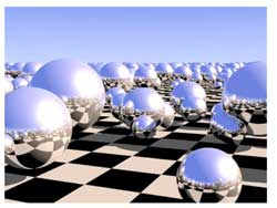
I’ve browsed the Google-pictures a bit and a picture
coming close to my mental image of the noncommutative manifold of a
Riemann surface locally looks like the picture on the left. Here, the checkerboard-surface is part of the Riemann surface
and the extra structure consists in putting in each point of the Riemann
surface a sphere, reflecting the local structure of the Riemann surface
near the point. In fact, my picture is slightly different : I want to
draw a loop in each point of the Riemann surface, but Ill explain why
the two pictures are equivalent and why they present a solution to the
problem of classifying all finite dimensional representations of the
Riemann surface. After all why do we draw and study Riemann
surfaces? Because we are interested in the solutions to equations. For
example, the points of the _Kleinian quartic Riemann
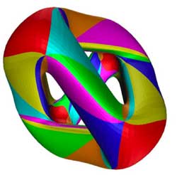
surface_ give us all solutions tex \in
\mathbb{C}^3 $ to the equation $X^3Y+Y^3Z+Z^3X=0 $. If (a,b,c) is such
a solution, then so are all scalar multiples $(\lambda a,\lambda
b,\lambda c) $ so we may as well assume that the Z$coordinate is equal
to 1 and are then interested in finding the solutions tex \in
\mathbb{C}^2 $ to the equation $X^3Y+Y^3+X=0 $ which gives us an affine
patch of the Kleinian quartic (in fact, these solutions give us all
points except for two, corresponding to the _points at infinity_ needed
to make the picture compact so that we can hold it in our hand and look
at it from all sides. These points at infinity correspond to the trivial
solutions (1,0,0) and (0,1,0)).

What is the connection
between points on this Riemann surface and representations? Well, if
(a,b) is a solution to the equation $X^3Y+Y^3+X=0 $, then we have a
_one-dimensional representation_ of the affine _coordinate ring_
$\mathbb{C}[X,Y]/(X^3Y+Y^3+X) $, that is, an algebra
morphism

$\mathbb{C}[X,Y]/(X^3Y+Y^3+X) \rightarrow \mathbb{C} $

defined by sending X to a and Y to b.
Conversely, any such one-dimensonal representation gives us a solution
(look at the images of X and Y and these will be the coordinates of
a solution). Thus, commutative algebraic geometry of smooth
curves (that is Riemann surfaces if you look at the ‘real’ picture)
can be seen as the study of one-dimensional representations of their
smooth coordinate algebras. In other words, the classical Riemann
surface gives us already the classifcation of all one-dimensional
representations, so now we are after the ‘other ones’.

In
noncommtative algebra it is not natural to restrict attention to algebra
maps to $\mathbb{C} $, at least we would also like to include algebra
maps to $n \times n $ matrices $M_n(\mathbb{C}) $. An n-dimensional
representation of the coordinate algebra of the Klein quartic is an
algebra map

$\mathbb{C}[X,Y]/(X^3Y+Y^3+X) \rightarrow M_n(\mathbb{C}) $

That is, we want to find all pairs of $n \times n $ matrices A and B satisfying the following
matrix-identities

$A.B=B.A $ and $A^3.B+B^3+A=0_n $

The
first equation tells us that the two matrices must commute (because we
took commuting variables X and Y) and the second equation really is
a set of $n^2 $-equations in the matrix-entries of A and
B.

There is a sneaky way to get lots of such matrix-couples
from a given solution (A,B), namely by _simultaneous conjugation_.
That is, if $C \in GL_n(\mathbb{C}) $ is any invertible $n \times n $
matrix, then also the matrix-couple $~(C^{-1}.A.C,C^{-1}.B.C) $
satisfies all the required equations (write the equations out and notice
that middle terms of the form $C.C^{-1} $ cancel out and check that one
then obtains the matrix-identities

$C^{-1} A B C = C^{-1} BA C $ and $C^{-1}(A^3B+B^3+A)C = 0_n $

which are satisfied because
(A,B) was supposed to be a solution). We then say that these two
n-dimensional representations are _isomorphic_ and naturally we are
only interested in classifying the isomorphism classes of all
representations.

Using classical commutative algebra theory of
Dedekind domains (such as the coordinate ring $\mathbb{C}[X,Y]/(X^3Y+Y^3+X) $)
allows us to give a complete solution to this problem. It says that any
n-dimensional representation is determined up to isomorphism by the
following geometric/combinatorial data

a finite set of points $P_1,P_2,\dots,P_k $ on the Riemann surface with $k \leq n $.
a set of positive integers $a_1,a_2,\dots,a_k $ associated to these pointssatisfying $a_1+a_2+\dots_a_k=n $.
for each $a_i $ a partition of $a_i $ (that is, a decreasing sequence of numbers with total sum
$a_i $).

To encode this classification I’ll use the mental
picture of associating to every point of the Klein quartic a small
loop. $\xymatrix{\vtx{}
\ar@(ul,ur)} $ Don\’t get over-exited about this
noncommutative manifold picture of the Klein quartic, I do not mean to
represent something like closed strings emanating from all points of the
Riemann surface or any other fanshi-wanshi interpretation. Just as
Feynman-diagrams allow the initiated to calculate probabilities of
certain interactions, the noncommutative manifold allows the
initiated to classify finite dimensional representations.

Our
mental picture of the noncommutative manifold of the Klein quartic, that
is : the points of the Klein quartic together with a loop in each point,
will tell the initiated quite a few things, such as : The fact
that there are no arrows between distict points, tells us that the
classification problem splits into local problems in a finite number of
points. Technically, this encodes the fact that there are no nontrivial
extensions between different simples in the commutative case. This will
drastically change if we enter the noncommutative world…

The fact that there is one loop in each point, tells us that
the local classification problem in that point is the same as that of
classifying nilpotent matrices upto conjugation (which, by the Jordan
normal form result, are classified by partitions) Moreover,
the fact that there is one loop in each point tells us that the local
structure of simple representations near that point (that is, the points
on the Kleinian quartic lying nearby) are classified as the simple
representations of the polynmial algebra $\mathbb{C}[x] $ (which are the
points on the complex plane, giving the picture
of the Riemann sphere in each point reflecting the local
neighborhood of the point on the Klein quartic)

In general, the
noncommutative manifold associated to a noncommutative smooth algebra
will be of a similar geometric/combinatorial nature. Typically, it will
consist of a geometric collection of points and arrows and loops between
these points. This data will then allow us to reduce the classification
problem to that of _quiver-representations_ and will allow us to give
local descriptions of our noncommutative manifolds. Next time,
I’ll give the details in the first noncommutative example : the
skew-group algebra of a finite group of automorphisms on a Riemann
surface (such as the simple group $PSL_2(\mathbb{F}_7) $ acting on the
Klein quartic). Already in this case, some new phenomena will
appear…

ADDED : While writing this post
NetNewsWire informed me that over at Noncommutative Geometry they have a
post on a similar topic : What is a noncommutative space.

the cartographers’ groups (2)

Published March 15, 2007 by lieven

Fortunately,
there is a drastic shortcut to the general tree-argument of last time, due to
Roger Alperin. Recall that the Moebius
transformations corresponding to u resp. v send z resp. to

$-\frac{1}{z} $ and $\frac{1}{1-z} $

whence the Moebius transformation
corresponding to $v^{-1} $ send z to $1-\frac{1}{z} $.

Consider
the set $\mathcal{P} $ of all positive irrational real numbers and the
set $\mathcal{N} $ of all negative irrational real numbers and observe
that

$u(\mathcal{P}) \subset \mathcal{N} $ and
$v^{\pm}(\mathcal{N}) \subset \mathcal{P} $

We have to show
that no alternating word $w=(u)v^{\pm}uv^{\pm}u \dots v^{\pm}(u) $ in
u and $v^{\pm} $ can be the identity in $PSL_2(\mathbb{Z}) $.

If the
length of w is odd then either $w(\mathcal{P}) \subset
\mathcal{N} $ or $w(\mathcal{N}) \subset
\mathcal{P} $ depending on whether w starts with a u or with
a $v^{\pm} $ term. Either way, this proves that no odd-length word can
be the identity element in $PSL_2(\mathbb{Z}) $.

If the length of
the word w is even we can assume that $w = v^{\pm}uv^{\pm}u \dots
v^{\pm}u $ (if necessary, after conjugating with u we get to this form).

There are two subcases, either $w=v^{-1}uv^{\pm}u \dots
v^{\pm}u $ in which case $w(\mathcal{P}) \subset v^{-1}(\mathcal{N}) $
and this latter set is contained in the set of all positive irrational
real numbers which are strictly larger than one .

Or, $w=vuv^{\pm}u \dots v^{\pm}u $ in which case
$w(\mathcal{P}) \subset v(\mathcal{N}) $ and this set is contained in
the set of all positive irrational real numbers strictly smaller than
one .

Either way, this shows that w cannot be the identity
morphism on $\mathcal{P} $ so cannot be the identity element in
$PSL_2(\mathbb{Z}) $.
Hence we have proved that

$PSL_2(\mathbb{Z}) = C_2 \ast C_3 = \langle u,v : u^2=1=v^3 \rangle $

A
description of $SL_2(\mathbb{Z}) $ in terms of generators and relations
follows

$SL_2(\mathbb{Z}) = \langle U,V : U^4=1=V^6, U^2=V^3 \rangle $

It is not true that $SL_2(\mathbb{Z}) $ is the free
product $C_4 \ast C_6 $ as there is the extra relation $U^2=V^3 $.

This relation says that the cyclic groups $C_4 = \langle U \rangle $
and $C_6 = \langle V \rangle $ share a common subgroup $C_2 = \langle
U^2=V^3 \rangle $ and this extra condition is expressed by saying that
$SL_2(\mathbb{Z}) $ is the amalgamated free product of $C_4 $ with
$C_6 $, amalgamated over the common subgroup $C_2 $ and denoted
as

$SL_2(\mathbb{Z}) = C_4 \ast_{C_2} C_6 $

More
generally, if G and H are finite groups, then the free product $G
\ast H $ consists of all words of the form $~(g_1)h_1g_2h_2g_3
\dots g_nh_n(g_{n-1}) $ (so alternating between non-identity
elements of G and H) and the group-law is induced by concatenation
of words (and group-laws in either G or H when end terms are
elements in the same group).

For example, take the dihedral groups $D_4
= \langle U,R : U^4=1=R^2,(RU)^2=1 \rangle $ and $D_6 = \langle V,S :
V^6=1=S^2,(SV)^2=1 \rangle $ then the free product can be expressed
as

$D_4 \ast D_6 = \langle U,V,R,S :
U^4=1=V^6=R^2=S^2=(RV)^2=(RU)^2 \rangle $

This almost fits in with
our obtained description of
$GL_2(\mathbb{Z}) $

$GL_2(\mathbb{Z}) = \langle U,V,R :
U^4=1=V^6=R^2=(RU)^2=(RV)^2, U^2=V^3 \rangle $

except for the
extra relations $R=S $ and $U^2=V^3 $ which express the fact that we
demand that $D_4 $ and $D_6 $ have the same subgroup

$D_2 = \langle U^2=V^3,S=R \rangle $

So, again we can express these relations by
saying that $GL_2(\mathbb{Z}) $ is the amalgamated free product of
the subgroups $D_4 = \langle U,R \rangle $ and $D_6 = \langle V,R
\rangle $, amalgamated over the common subgroup $D_2 = C_2 \times C_2 =
\langle U^2=V^3,R \rangle $. We write

$GL_2(\mathbb{Z}) = D_4
\ast_{D_2} D_6 $

Similarly (but a bit easier) for
$PGL_2(\mathbb{Z}) $ we have

$PGL_2(\mathbb{Z}) = \langle u,v,R: u^2=v^3=1=R^2 = (Ru)^2 = (Rv)^2 \rangle $

which can be seen as
the amalgamated free product of $D_2 = \langle u,R \rangle $ with $D_3
= \langle v,R \rangle $, amalgamated over the common subgroup $C_2 =
\langle R \rangle $ and therefore

$PGL_2(\mathbb{Z}) = D_2
\ast_{C_2} D_3 $

Now let us turn to congruence subgroups of
the modular group.
With $\Gamma(n) $ one denotes the kernel of the natural
surjection

$PSL_2(\mathbb{Z}) \rightarrow
PSL_2(\mathbb{Z}/n\mathbb{Z}) $

that is all elements represented by a matrix

$\begin{bmatrix} a
& b \\ c & d \end{bmatrix} $

such that a=d=1 (mod n) and b=c=0
(mod n). On the other hand $\Gamma_0(n) $ consists of elements
represented by matrices such that only c=0 (mod n). Both are finite
index subgroups of $PSL_2(\mathbb{Z}) $.

As we have seen that
$PSL_2(\mathbb{Z}) = C_2 \ast C_3 $ it follows from general facts
on free products that any finite index subgroup is of the
form

$C_2 \ast C_2 \ast \dots \ast C_2 \ast
C_3 \ast C_3 \ast \dots \ast C_3 \ast C_{\infty}
\ast C_{\infty} \dots \ast C_{\infty} $

that is the
free product of k copies of $C_2 $, l copies of $C_3 $ and m copies
of $C_{\infty} $ where it should be noted that k,l and m are allowed
to be zero. There is an elegant way to calculate explicit generators of
these factors for congruence subgroups, due to Ravi S. Kulkarni (An
Arithmetic-Geometric Method in the Study of the Subgroups of the Modular
Group , American Journal of Mathematics, Vol. 113, No. 6. (Dec.,
1991), pp. 1053-1133) which deserves another (non-course) post.

Using this method one finds that $\Gamma_0(2) $ is generated by
the Moebius transformations corresponding to the
matrices

$X=\begin{bmatrix} 1 & 1 \\ 0 & 1 \end{bmatrix} $ and
$Y=\begin{bmatrix} 1 & -1 \\ 2 & -1 \end{bmatrix} $

and that
generators for $\Gamma(2) $ are given by the
matrices

$A=\begin{bmatrix} 1 & 0 \\ -2 & 1 \end{bmatrix} $
and $B=\begin{bmatrix} 1 & -2 \\ 2 & -3 \end{bmatrix} $

Next,
one has to write these generators in terms of the generating matrices
u and v of $PSL_2(\mathbb{Z}) $ and as we know all relations between
u and v the relations of these congruence subgroups will follow.

We
will give the details for $\Gamma_0(2) $ and leave you to figure out
that $\Gamma(2) = C_{\infty} \ast C_{\infty} $ (that is that
there are no relations between the matrices A and
B).

Calculate that $X=v^2u $ and that $Y=vuv^2 $. Because the
only relations between u and v are $v^3=1=u^2 $ we see that Y is an
element of order two as $Y^2 = vuv^3uv^2= v^3 = 1 $ and that no power of
X can be the identity transformation.

But then also none of the
elements $~(Y)X^{i_1}YX^{i_2}Y \dots YX^{i_n}(Y) $ can be the identity
(write it out as a word in u and v) whence,
indeed

$\Gamma_0(2) = C_{\infty} \ast C_2 $

In fact,
the group $\Gamma_0(2) $ is staring you in the face whenever you come to
this site. I fear I’ve never added proper acknowledgements for the
beautiful header-picture

so I’d better do it now. The picture is due to Helena
Verrill and she has a
page with
more pictures. The header-picture depicts a way to get a fundamental
domain for the action of $\Gamma_0(2) $ on the upper half plane. Such a
fundamental domain consists of any choice of 6 tiles with different
colours (note that there are two shades of blue and green). Helena also
has a
Java-applet
to draw fundamental domains of more congruence subgroups.

The cartographers’ groups

Published March 13, 2007 by lieven

Just as cartographers like
Mercator drew maps of
the then known world, we draw dessins
d ‘enfants to depict the
associated algebraic curve defined over
$\overline{\mathbb{Q}} $.

In order to see that such a dessin
d’enfant determines a permutation representation of one of
Grothendieck’s cartographic groups, $SL_2(\mathbb{Z}),
\Gamma_0(2) $ or $\Gamma(2) $ we need to have realizations of these
groups (as well as their close relatives
$PSL_2(\mathbb{Z}),GL_2(\mathbb{Z}) $ and $PGL_2(\mathbb{Z}) $) in
terms of generators and relations.

As this lesson will be rather
technical I’d better first explain what we will prove (so that you can
skip it if you feel comfortable with the statements) and why we want to
prove it. What we will prove in detail below is that these groups
can be written as free (or amalgamated) group products. We will explain
what this means and will establish that

$PSL_2(\mathbb{Z}) = C_2
\ast C_3, \Gamma_0(2) = C_2 \ast C_{\infty}, \Gamma(2)
= C_{\infty} \ast C_{\infty} $

$SL_2(\mathbb{Z}) =
C_4 \ast_{C_2} C_6, GL_2(\mathbb{Z}) = D_4 \ast_{D_2} D_6,
PGL_2(\mathbb{Z}) = D_2 \ast_{C_2} D_3 $

where $C_n $ resp.
$D_n $ are the cyclic (resp. dihedral) groups. The importance of these
facts it that they will allow us to view the set of (isomorphism classes
of) finite dimensional representations of these groups as
noncommutative manifolds . Looking at the statements above we
see that these arithmetical groups can be build up from the first
examples in any course on finite groups : cyclic and dihedral
groups.

Recall that the cyclic group of order n, $C_n $ is the group of
rotations of a regular n-gon (so is generated by a rotation r with
angle $\frac{2 \pi}{n} $ and has defining relation $r^n = 1 $, where 1
is the identity). However, regular n-gons have more symmetries :
flipping over one of its n lines of symmetry

The dihedral group $D_n $ is the group generated by the n
rotations and by these n flips. If, as before r is a generating
rotation and d is one of the flips, then it is easy to see that the
dihedral group is generated by r and d and satisfied the defining
relations

$r^n=1 $ and $d^2 = 1 = (rd)^2 $

Flipping twice
does nothing and to see the relation $~(rd)^2=1 $ check that doing twice a
rotation followed by a flip brings all vertices back to their original
location. The dihedral group $D_n $ has 2n elements, the n-rotations
$r^i $ and the n flips $dr^i $.

In fact, to get at the cartographic
groups we will only need the groups $D_4, D_6 $ and their
subgroups. Let us start by finding generators of the largest
group $GL_2(\mathbb{Z}) $ which is the group of all invertible $2
\times 2 $ matrices with integer coefficients.

Consider the
elements

$U = \begin{bmatrix} 0 & -1 \\ 1 & 0 \end{bmatrix},
V = \begin{bmatrix} 0 & 1 \\ -1 & 1 \end{bmatrix}/tex] and $R =
\begin{bmatrix} 0 & 1 \\ 1 & 0 \end{bmatrix} $

and form the
matrices

$X = UV = \begin{bmatrix} 1 & -1 \\ 0 & 1
\end{bmatrix}, Y = VU = \begin{bmatrix} 1 & 0 \\ 1 & 1
\end{bmatrix} $

By induction we prove the following relations in
$GL_2(\mathbb{Z}) $

$X^n \begin{bmatrix} a & b \\ c & d
\end{bmatrix} = \begin{bmatrix} a-nc & b-nd \\ c & d \end{bmatrix} $
and $\begin{bmatrix} a & b \\ c& d \end{bmatrix} X^n =
\begin{bmatrix} a & b-na \\ c & d-nc \end{bmatrix} $

$Y^n \begin{bmatrix} a & b \\ c & d \end{bmatrix} =
\begin{bmatrix} a & b \\ c+na & d+nb \end{bmatrix} $ and
$\begin{bmatrix} a & b \\ c & d \end{bmatrix} Y^n = \begin{bmatrix}
a+nb & b \\ c+nd & d \end{bmatrix} $

The determinant ad-bc of
a matrix in $GL_2(\mathbb{Z}) $ must be $\pm 1 $ whence all rows and
columns of

$\begin{bmatrix} a & b \\ c & d \end{bmatrix} \in
GL_2(\mathbb{Z}) $

consist of coprime numbers and hence a and
c can be reduced modulo each other by left multiplication by a power
of X or Y until one of them is zero and the other is $\pm 1 $. We
may even assume that $a = \pm 1 $ (if not, left multiply with U).

So,
by left multiplication by powers of X and Y and U we can bring any
element of $GL_2(\mathbb{Z}) $ into the form

$\begin{bmatrix}
\pm 1 & \beta \\ 0 & \pm 1 \end{bmatrix} $

and again by left
multiplication by a power of X we can bring it in one of the four
forms

$\begin{bmatrix} \pm 1 & 0 \\ 0 & \pm 1 \end{bmatrix}
= { 1,UR,RU,U^2 } $

This proves that $GL_2(\mathbb{Z}) $ is
generated by the elements U,V and R.

Similarly, the group
$SL_2(\mathbb{Z}) $ of all $2 \times 2 $ integer matrices with
determinant 1 is generated by the elements U and V as using the
above method and the restriction on the determinant we will end up with
one of the two matrices

${ \begin{bmatrix} 1 & 0 \\ 0 & 1
\end{bmatrix},\begin{bmatrix} -1 & 0 \\ 0 & -1 \end{bmatrix} } =
{ 1,U^2 } $

so we never need the matrix R. As for
relations, there are some obvious relations among the matrices U,V and
R, namely

$U^2=V^3 $ and $1=U^4=R^2=(RU)^2=(RV)^2$ $

The
real problem is to prove that all remaining relations are consequences
of these basic ones. As R clearly has order two and its commutation
relations with U and V are just $RU=U^{-1}R $ and $RV=V^{-1}R $ we can
pull R in any relation to the far right and (possibly after
multiplying on the right with R) are left to prove that the only
relations among U and V are consequences of $U^2=V^3 $ and
$U^4=1=V^6 $.

Because $U^2=V^3 $ this element is central in the
group generated by U and V (which we have seen to be
$SL_2(\mathbb{Z}) $) and if we quotient it out we get the modular
group

$\Gamma = PSL_2(\mathbb{Z}) $

Hence in order to prove our claim
it suffices that

$PSL_2(\mathbb{Z}) = \langle
\overline{U},\overline{V} : \overline{U}^2=\overline{V}^3=1
\rangle $

Phrased differently, we have to show that
$PSL_2(\mathbb{Z}) $ is the free group product of the cyclic groups of
order two and three (those generated by $u = \overline{U} $ and
$v=\overline{V} $) $C_2 \ast C_3 $

Any element of this free group
product is of the form $~(u)v^{a_1}uv^{a_2}u \ldots
uv^{a_k}(u) $ where beginning and trailing u are optional and
all $a_i $ are either 1 or 2.

So we have to show that in
$PSL_2(\mathbb{Z}) $ no such word can give the identity
element. Today, we will first sketch the classical argument based
on the theory of groups acting on trees due to Jean-Pierre
Serre and Hyman Bass. Tomorrow, we will give a short elegant proof due to
Roger Alperin and draw
consequences to the description of the carthographic groups as
amalgamated free products of cyclic and dihedral groups.

Recall
that $GL_2(\mathbb{Z}) $ acts via Moebius
transformations on
the complex plane $\mathbb{C} = \mathbb{R}^2 $ (actually it is an
action on the Riemann sphere $\mathbb{P}^1_{\mathbb{C}} $) given by the
maps

$\begin{bmatrix} a & b \\ c & d \end{bmatrix}.z =
\frac{az+b}{cz+d} $

Note that the action of the
center of $GL_2(\mathbb{Z}) $ (that is of $\pm \begin{bmatrix} 1 & 0
\\ 0 & 1 \end{bmatrix} $) acts trivially, so it is really an action of
$PGL_2(\mathbb{Z}) $.

As R interchanges the upper and lower half-plane
we might as well restrict to the action of $SL_2(\mathbb{Z}) $ on the
upper-halfplane $\mathcal{H} $. It is quite easy to see that a
fundamental domain
for this action is given by the greyed-out area

To see that any $z \in \mathcal{H} $ can be taken into this
region by an element of $PSL_2(\mathbb{Z}) $ note the following two
Moebius transformations

$\begin{bmatrix} 1 & 1 \\ 0 & 1
\end{bmatrix}.z = z+1 $ and $\begin{bmatrix} 0 & 1 \\ -1
& 0 \end{bmatrix}.z = -\frac{1}{z} $

The first
operation takes any z into a strip of length one, for example that
with Re(z) between $-\frac{1}{2} $ and $\frac{1}{2} $ and the second
interchanges points within and outside the unit-circle, so combining the
two we get any z into the greyed-out region. Actually, we could have
taken any of the regions in the above tiling as our fundamental domain
as they are all translates of the greyed-out region by an element of
$PSL_2(\mathbb{Z}) $.

Of course, points on the boundary of the
greyed-out fundamental region need to be identified (in order to get the
identification of $\overline{\mathcal{H}/PSL_2(\mathbb{Z})} $ with the
Riemann sphere $S^2=\mathbb{P}^1_{\mathbb{C}} $). For example, the two
halves of the boundary by the unit circle are interchanged by the action
of the map $z \rightarrow -\frac{1}{z} $ and if we take the translates under
$PSL_2(\mathbb{Z}) $ of the indicated circle-part

we get a connected tree with fundamental domain the circle
part bounded by i and $\rho = \frac{1}{2}+\frac{\sqrt{3}}{2} i $.
Calculating the stabilizer subgroup of i (that is, the subgroup of
elements fixing i) we get that this subgroup
is $\langle u \rangle = C_2 $ whereas the stabilizer subgroup of
$\rho $ is $\langle v \rangle = C_3 $.

Using this facts and the general
results of Jean-Pierre Serres book Trees
one deduces that $PSL_2(\mathbb{Z}) = C_2 \ast C_3 $
and hence that the obvious relations among U,V and R given above do
indeed generate all relations.