Category: featured

anabelian geometry

Published March 22, 2007 by lieven

Last time we saw
that a curve defined over $\overline{\mathbb{Q}} $ gives rise
to a permutation representation of $PSL_2(\mathbb{Z}) $ or one
of its subgroups $\Gamma_0(2) $ (of index 2) or
$\Gamma(2) $ (of index 6). As the corresponding
monodromy group is finite, this representation factors through a normal
subgroup of finite index, so it makes sense to look at the profinite
completion of $SL_2(\mathbb{Z}) $, which is the inverse limit
of finite
groups $\underset{\leftarrow}{lim}~SL_2(\mathbb{Z})/N $
where N ranges over all normalsubgroups of finite index. These
profinte completions are horrible beasts even for easy groups such as
$\mathbb{Z} $. Its profinite completion
is

$\underset{\leftarrow}{lim}~\mathbb{Z}/n\mathbb{Z} =
\prod_p \hat{\mathbb{Z}}_p $

where the right hand side
product of p-adic integers ranges over all prime numbers! The
_absolute Galois group_
$G=Gal(\overline{\mathbb{Q}}/\mathbb{Q}) $ acts on all curves
defined over $\overline{\mathbb{Q}} $ and hence (via the Belyi
maps ans the corresponding monodromy permutation representation) there
is an action of $G $ on the profinite completions of the
carthographic groups.

This is what Grothendieck calls anabelian
algebraic geometry

Returning to the general
case, since finite maps can be interpreted as coverings over
$\overline{\mathbb{Q}} $ of an algebraic curve defined over
the prime field $~\mathbb{Q} $ itself, it follows that the
Galois group $G $ of $\overline{\mathbb{Q}} $ over
$~\mathbb{Q} $ acts on the category of these maps in a
natural way.
For instance, the operation of an automorphism
$~\gamma \in G $ on a spherical map given by the rational
function above is obtained by applying $~\gamma $ to the
coefficients of the polynomials P , Q. Here, then, is that
mysterious group $G $ intervening as a transforming agent on
topologico- combinatorial forms of the most elementary possible
nature, leading us to ask questions like: are such and such oriented
maps ‚conjugate or: exactly which are the conjugates of a given
oriented map? (Visibly, there is only a finite number of these).
I considered some concrete cases (for coverings of low degree) by
various methods, J. Malgoire considered some others ‚ I doubt that
there is a uniform method for solving the problem by computer. My
reflection quickly took a more conceptual path, attempting to
apprehend the nature of this action of G.
One sees immediately
that roughly speaking, this action is expressed by a certain
outer action of G on the profinite com- pactification of the
oriented cartographic group $C_+^2 = \Gamma_0(2) $ , and this
action in its turn is deduced by passage to the quotient of the
canonical outer action of G on the profinite fundamental group
$\hat{\pi}_{0,3} $ of
$(U_{0,3})_{\overline{\mathbb{Q}}} $ where
$U_{0,3} $ denotes the typical curve of genus 0 over the
prime field Q, with three points re- moved.
This is how my
attention was drawn to what I have since termed anabelian
algebraic geometry, whose starting point was exactly a study
(limited for the moment to characteristic zero) of the action of
absolute Galois groups (particularly the groups Gal(K/K),
where K is an extension of finite type of the prime field) on
(profinite) geometric fundamental groups of algebraic varieties
(defined over K), and more particularly (break- ing with a
well-established tradition) fundamental groups which are very far
from abelian groups (and which for this reason I call
anabelian).
Among these groups, and very close to
the group $\hat{\pi}_{0,3} $ , there is the profinite
compactification of the modular group $Sl_2(\mathbb{Z}) $,
whose quotient by its centre ±1 contains the former as congruence
subgroup mod 2, and can also be interpreted as an oriented
cartographic group, namely the one classifying triangulated
oriented maps (i.e. those whose faces are all triangles or
monogons).

and a bit further, on page
250

I would like to conclude this rapid outline
with a few words of commentary on the truly unimaginable richness
of a typical anabelian group such as $SL_2(\mathbb{Z}) $
doubtless the most remarkable discrete infinite group ever
encountered, which appears in a multiplicity of avatars (of which
certain have been briefly touched on in the present report), and which
from the point of view of Galois-Teichmuller theory can be
considered as the fundamental ‚building block‚ of the
Teichmuller tower
The element of the structure of
$Sl_2(\mathbb{Z}) $ which fascinates me above all is of course
the outer action of G on its profinite compactification. By
Bielyi’s theorem, taking the profinite compactifications of subgroups
of finite index of $Sl_2(\mathbb{Z}) $, and the induced
outer action (up to also passing to an open subgroup of G), we
essentially find the fundamental groups of all algebraic curves (not
necessarily compact) defined over number fields K, and the outer
action of $Gal(\overline{K}/K) $ on them at least it is
true that every such fundamental group appears as a quotient of one
of the first groups.
Taking the anabelian yoga
(which remains conjectural) into account, which says that an anabelian
algebraic curve over a number field K (finite extension of Q) is
known up to isomorphism when we know its mixed fundamental group (or
what comes to the same thing, the outer action of
$Gal(\overline{K}/K) $ on its profinite geometric
fundamental group), we can thus say that
all algebraic
curves defined over number fields are contained in the profinite
compactification $\widehat{SL_2(\mathbb{Z})} $ and in the
knowledge of a certain subgroup G of its group of outer
automorphisms!

To study the absolute
Galois group $Gal(\overline{\mathbb{\mathbb{Q}}}/\mathbb{Q}) $ one
investigates its action on dessins denfants. Each dessin will be part of
a finite family of dessins which form one orbit under the Galois action
and one needs to find invarians to see whether two dessins might belong
to the same orbit. Such invariants are called _Galois invariants_ and
quite a few of them are known.

Among these the easiest to compute
are

the valency list of a dessin : that is the valencies of all
vertices of the same type in a dessin
the monodromy group of a dessin : the subgroup of the symmetric group $S_d $ where d is
the number of edges in the dessin generated by the partitions $\tau_0 $
and $\tau_1 $ For example, we have seen
before that the two
Mathieu-dessins

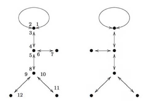
form a Galois orbit. As graphs (remeber we have to devide each
of the edges into two and the midpoints of these halfedges form one type
of vertex, the other type are the black vertices in the graphs) these
are isomorphic, but NOT as dessins as we have to take the embedding of
them on the curve into account. However, for both dessins the valency
lists are (white) : (2,2,2,2,2,2) and (black) :
(3,3,3,1,1,1) and one verifies that both monodromy groups are
isomorphic to the Mathieu simple group $M_{12} $ though they are
not conjugated as subgroups of $S_{12} $.

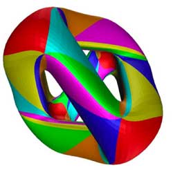
Recently, new
Galois invariants were obtained from physics. In Children’s drawings
from Seiberg-Witten curves
the authors argue that there is a close connection between Grothendiecks
programme of classifying dessins into Galois orbits and the physics
problem of classifying phases of N=1 gauge theories…

Apart
from curves defined over $\overline{\mathbb{Q}} $ there are
other sources of semi-simple $SL_2(\mathbb{Z}) $
representations. We will just mention two of them and may return to them
in more detail later in the course.

Sporadic simple groups and
their representations There are 26 exceptional finite simple groups
and as all of them are generated by two elements, there are epimorphisms
$\Gamma(2) \rightarrow S $ and hence all their representations
are also semi-simple $\Gamma(2) $-representations. In fact,
looking at the list of ‘standard generators’ of the sporadic
simples

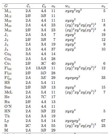
(here the conjugacy classes of the generators follow the
notation of the Atlas project) we see that all but
possibly one are epimorphic images of $\Gamma_0(2) = C_2 \ast
C_{\infty} $ and that at least 12 of then are epimorphic images
of $PSL_2(\mathbb{Z}) = C_2 \ast
C_3 $.

Rational conformal field theories Another
source of $SL_2(\mathbb{Z}) $ representations is given by the
modular data associated to rational conformal field theories.

These
representations also factor through a quotient by a finite index normal
subgroup and are therefore again semi-simple
$SL_2(\mathbb{Z}) $-representations. For a readable
introduction to all of this see chapter 6 \”Modular group
representations throughout the realm\” of the
book Moonshine beyond the monster the bridge connecting algebra, modular forms and physics by Terry
Gannon. In fact, the whole book
is a good read. It introduces a completely new type of scientific text,
that of a neverending survey paper…

permutation representations of monodromy groups

Published March 20, 2007 by lieven

Today we will explain how curves defined over
$\overline{\mathbb{Q}} $ determine permutation representations
of the carthographic groups. We have seen that any smooth projective
curve $C $ (a Riemann surface) defined over the algebraic
closure $\overline{\mathbb{Q}} $ of the rationals, defines a
_Belyi map_ $\xymatrix{C \ar[rr]^{\pi} & & \mathbb{P}^1} $ which is only ramified over the three points
$\\{ 0,1,\infty \\} $. By this we mean that there are
exactly $d $ points of $C $ lying over any other point
of $\mathbb{P}^1 $ (we call $d $ the degree of
$\pi $) and that the number of points over $~0,1~ $ and
$~\infty $ is smaller than $~d $. To such a map we
associate a _dessin d\’enfant_, a drawing on $C $ linking the
pre-images of $~0 $ and $~1 $ with exactly $d $
edges (the preimages of the open unit-interval). Next, we look at
the preimages of $~0 $ and associate a permutation
$\tau_0 $ of $~d $ letters to it by cycling
counter-clockwise around these preimages and recording the edges we
meet. We repeat this procedure for the preimages of $~1 $ and
get another permutation $~\tau_1 $. That is, we obtain a
subgroup of the symmetric group $ \langle \tau_0,\tau_1
\rangle \subset S_d $ which is called the monodromy
group of the covering $\pi $.

For example, the
dessin on the right is
associated to a degree $8 $ map $\mathbb{P}^1 \rightarrow
\mathbb{P}^1 $ and if we let the black (resp. starred) vertices be
the preimages of $~0 $ (respectively of $~1 $), then the
corresponding partitions are $\tau_0 = (2,3)(1,4,5,6) $
and $\tau_1 = (1,2,3)(5,7,8) $ and the monodromy group
is the alternating group $A_8 $ (use
GAP ).

But wait! The map is also
ramified in $\infty $ so why don\’t we record also a
permutation $\tau_{\infty} $ and are able to compute it from
the dessin? (Note that all three partitions are needed if we want to
reconstruct $C $ from the $~d $ sheets as they encode in
which order the sheets fit together around the preimages). Well,
the monodromy group of a $\mathbb{P}^1 $ covering ramified only
in three points is an epimorphic image of the fundamental
group of the sphere
minus three points $\pi_1(\mathbb{P}^1 – { 0,1,\infty
}) $ That is, the group of all loops beginning and
ending in a basepoint upto homotopy (that is, two such loops are the
same if they can be transformed into each other in a continuous way
while avoiding the three points).

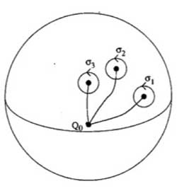
This group is generated by loops
$\sigma_i $ running from the basepoint to nearby the i-th
point, doing a counter-clockwise walk around it and going back to be
basepoint $Q_0 $ and the epimorphism to the monodromy group is given by sending

$\sigma_1 \mapsto \tau_0~\quad~\sigma_2 \mapsto
\tau_1~\quad~\sigma_3 \mapsto \tau_{\infty} $

Now,
these three generators are not independent. In fact, this fundamental
group is

$\pi_1(\mathbb{P}^1 – \\{ 0,1,\infty \\}) =
\langle \sigma_1,\sigma_2,\sigma_3~\mid~\sigma_1 \sigma_2
\sigma_3 = 1 \rangle $

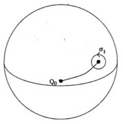
To understand this, let us begin
with an easier case, that of the sphere minus one point. The fundamental group of the plane minus one point is
$~\mathbb{Z} $ as it encodes how many times we walk around the
point. However, on the sphere the situation is different as we can make
our walk around the point longer and longer until the whole walk is done
at the backside of the sphere and then we can just contract our walk to
the basepoint. So, there is just one type of walk on a sphere minus one
point (upto homotopy) whence this fundamental group is trivial. Next,
let us consider the sphere minus two points

Repeat the foregoing to the walk $\sigma_2 $, that
is, strech the upper part of the circular tour all over the backside of
the sphere and then we see that we can move it to fit with the walk
$\sigma_1$ BUT for the orientation of the walk! That is, if we do this
modified walk $\sigma_1 \sigma_2^{\’} $ we just made the
trivial walk. So, this fundamental group is $\langle
\sigma_1,\sigma_2~\mid~\sigma_1 \sigma_2 = 1 \rangle =
\mathbb{Z} $ This is also the proof of the above claim. For,
we can modify the third walk $\sigma_3 $ continuously so that
it becomes the walk $\sigma_1 \sigma_2 $ but
with the reversed orientation ! As $\sigma_3 =
(\sigma_1 \sigma_2)^{-1} $ this allows us to compute the
\’missing\’ permutation $\tau_{\infty} = (\tau_0
\tau_1)^{-1} $ In the example above, we obtain
$\tau_{\infty}= (1,2,6,5,8,7,4)(3) $ so it has two cycles
corresponding to the fact that the dessin has two regions (remember we
should draw ths on the sphere) : the head and the outer-region. Hence,
the pre-images of $\infty$ correspond to the different regions of the
dessin on the curve $C $. For another example,
consider the degree 168 map

$K \rightarrow \mathbb{P}^1 $

which is the modified orbit map for the action of
$PSL_2(\mathbb{F}_7) $ on the Klein quartic.
The corresponding dessin is the heptagonal construction of the Klein
quartic

Here, the pre-images of 1 correspond to the midpoints of the
84 edges of the polytope whereas the pre-images of 0 correspond to the
56 vertices. We can label the 168 half-edges by numbers such that
$\tau_0 $ and $\tau_1 $ are the standard generators b
resp. a of the 168-dimensional regular representation (see the atlas
page ).
Calculating with GAP the element $\tau_{\infty} = (\tau_0
\tau_1)^{-1} = (ba)^{-1} $ one finds that this permutation
consists of 24 cycles of length 7, so again, the pre-images of
$\infty $ lie one in each of the 24 heptagonal regions of the
Klein quartic. Now, we are in a position to relate curves defined
over $\overline{Q} $ via their Belyi-maps and corresponding
dessins to Grothendiecks carthographic groups $\Gamma(2) $,
$\Gamma_0(2) $ and $SL_2(\mathbb{Z}) $. The
dessin gives a permutation representation of the monodromy group and
because the fundamental group of the sphere minus three
points $\pi_1(\mathbb{P}^1 – \\{ 0,1,\infty \\}) =
\langle \sigma_1,\sigma_2,\sigma_3~\mid~\sigma_1 \sigma_2
\sigma_3 = 1 \rangle = \langle \sigma_1,\sigma_2
\rangle $ is the free group op two generators, we see that
any dessin determines a permutation representation of the congruence
subgroup $\Gamma(2) $ (see this
post where we proved that this
group is free). A clean dessin is one for which one type of
vertex has all its valancies (the number of edges in the dessin meeting
the vertex) equal to one or two. (for example, the pre-images of 1 in
the Klein quartic-dessin or the pre-images of 1 in the monsieur Mathieu
example ) The corresponding
permutation $\tau_1 $ then consists of 2-cycles and hence the
monodromy group gives a permutation representation of the free
product $C_{\infty} \ast C_2 =
\Gamma_0(2) $ Finally, a clean dessin is said to be a
quilt dessin if also the other type of vertex has all its valancies
equal to one or three (as in the Klein quartic or Mathieu examples).
Then, the corresponding permutation has order 3 and for these
quilt-dessins the monodromy group gives a permutation representation of
the free product $C_2 \ast C_3 =
PSL_2(\mathbb{Z}) $ Next time we will see how this lead
Grothendieck to his anabelian geometric approach to the absolute Galois
group.

noncommutative curves and their maniflds

Published March 17, 2007 by lieven

Last time we have
seen that the noncommutative manifold of a Riemann surface can be viewed
as that Riemann surface together with a loop in each point. The extra
loop-structure tells us that all finite dimensional representations of
the coordinate ring can be found by separating over points and those
living at just one point are classified by the isoclasses of nilpotent
matrices, that is are parametrized by the partitions (corresponding
to the sizes of the Jordan blocks). In addition, these loops tell us
that the Riemann surface locally looks like a Riemann sphere, so an
equivalent mental picture of the local structure of this
noncommutative manifold is given by the picture on teh left, where the surface is part of the Riemann surface
and a sphere is placed at every point. Today we will consider
genuine noncommutative curves and describe their corresponding
noncommutative manifolds.

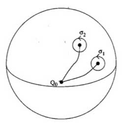
Here, a mental picture of such a
_noncommutative sphere_ to keep in mind would be something
like the picture on the right. That is, in most points of the sphere we place as before again
a Riemann sphere but in a finite number of points a different phenomen
occurs : we get a cluster of infinitesimally nearby points. We
will explain this picture with an easy example. Consider the
complex plane $\mathbb{C} $, the points of which are just the
one-dimensional representations of the polynomial algebra in one
variable $\mathbb{C}[z] $ (any algebra map $\mathbb{C}[z] \rightarrow \mathbb{C} $ is fully determined by the image of z). On this plane we
have an automorphism of order two sending a complex number z to its
negative -z (so this automorphism can be seen as a point-reflexion
with center the zero element 0). This automorphism extends to
the polynomial algebra, again induced by sending z to -z. That
is, the image of a polynomial $f(z) \in \mathbb{C}[z] $ under this
automorphism is f(-z).

With this data we can form a noncommutative
algebra, the _skew-group algebra_ $\mathbb{C}[z] \ast C_2 $ the
elements of which are either of the form $f(z) \ast e $ or $g(z) \ast g $ where
$C_2 = \langle g : g^2=e \rangle $ is the cyclic group of order two
generated by the automorphism g and f(z),g(z) are arbitrary
polynomials in z.

The multiplication on this algebra is determined by
the following rules

$(g(z) \ast g)(f(z) \ast e) = g(z)f(-z) \astg $ whereas $(f(z) \ast e)(g(z) \ast g) = f(z)g(z) \ast g $

$(f(z) \ast e)(g(z) \ast e) = f(z)g(z) \ast e $ whereas $(f(z) \ast g)(g(z)\ast g) = f(z)g(-z) \ast e $

That is, multiplication in the
$\mathbb{C}[z] $ factor is the usual multiplication, multiplication in
the $C_2 $ factor is the usual group-multiplication but when we want
to get a polynomial from right to left over a group-element we have to
apply the corresponding automorphism to the polynomial (thats why we
call it a _skew_ group-algebra).

Alternatively, remark that as
a $\mathbb{C} $-algebra the skew-group algebra $\mathbb{C}[z] \ast C_2 $ is
an algebra with unit element 1 = 1\aste and is generated by
the elements $X = z \ast e $ and $Y = 1 \ast g $ and that the defining
relations of the multiplication are

$Y^2 = 1 $ and $Y.X =-X.Y $

hence another description would
be

$\mathbb{C}[z] \ast C_2 = \frac{\mathbb{C} \langle X,Y \rangle}{ (Y^2-1,XY+YX) } $

It can be shown that skew-group
algebras over the coordinate ring of smooth curves are _noncommutative
smooth algebras_ whence there is a noncommutative manifold associated
to them. Recall from last time the noncommutative manifold of a
smooth algebra A is a device to classify all finite dimensional
representations of A upto isomorphism Let us therefore try to
determine some of these representations, starting with the
one-dimensional ones, that is, algebra maps from

$\mathbb{C}[z] \ast C_2 = \frac{\mathbb{C} \langle X,Y \rangle}{ (Y^2-1,XY+YX) } \rightarrow \mathbb{C} $

Such a map is determined by the image of X and that of
Y. Now, as $Y^2=1 $ we have just two choices for the image of Y
namely +1 or -1. But then, as the image is a commutative algebra
and as XY+YX=0 we must have that the image of 2XY is zero whence the
image of X must be zero. That is, we have only
two one-dimensional representations, namely $S_+ : X \rightarrow 0, Y \rightarrow 1 $
and $S_- : X \rightarrow 0, Y \rightarrow -1 $

This is odd! Can
it be that our noncommutative manifold has just 2 points? Of course not.
In fact, these two points are the exceptional ones giving us a cluster
of nearby points (see below) whereas most points of our
noncommutative manifold will correspond to 2-dimensional
representations!

So, let’s hunt them down. The
center of $\mathbb{C}[z]\ast C_2 $ (that is, the elements commuting with
all others) consists of all elements of the form $f(z)\ast e $ with f an
_even_ polynomial, that is, f(z)=f(-z) (because it has to commute
with 1\ast g), so is equal to the subalgebra $\mathbb{C}[z^2]\ast e $.

The
manifold corresponding to this subring is again the complex plane
$\mathbb{C} $ of which the points correspond to all one-dimensional
representations of $\mathbb{C}[z^2]\ast e $ (determined by the image of
$z^2\ast e $).

We will now show that to each point of $\mathbb{C} – { 0 } $
corresponds a simple 2-dimensional representation of
$\mathbb{C}[z]\ast C_2 $.

If a is not zero, we will consider the
quotient of the skew-group algebra modulo the twosided ideal generated
by $z^2\ast e-a $. It turns out
that

$\frac{\mathbb{C}[z]\ast C_2}{(z^2\aste-a)} =
\frac{\mathbb{C}[z]}{(z^2-a)} \ast C_2 = (\frac{\mathbb{C}[z]}{(z-\sqrt{a})}
\oplus \frac{\mathbb{C}[z]}{(z+\sqrt{a})}) \ast C_2 = (\mathbb{C}
\oplus \mathbb{C}) \ast C_2 $

where the skew-group algebra on the
right is given by the automorphism g on $\mathbb{C} \oplus \mathbb{C} $ interchanging the two factors. If you want to
become more familiar with working in skew-group algebras work out the
details of the fact that there is an algebra-isomorphism between
$(\mathbb{C} \oplus \mathbb{C}) \ast C_2 $ and the algebra of $2 \times 2 $ matrices $M_2(\mathbb{C}) $. Here is the
identification

$~(1,0)\aste \rightarrow \begin{bmatrix} 1 & 0 \\ 0 & 0 \end{bmatrix} $

$~(0,1)\aste \rightarrow \begin{bmatrix} 0 & 0 \\ 0 & 1 \end{bmatrix} $

$~(1,0)\astg \rightarrow \begin{bmatrix} 0 & 1 \\ 0 & 0 \end{bmatrix} $

$~(0,1)\astg \rightarrow \begin{bmatrix} 0 & 0 \\ 1 & 0 \end{bmatrix} $

so you have to verify that multiplication
on the left hand side (that is in $(\mathbb{C} \oplus \mathbb{C}) \ast
C_2 $) coincides with matrix-multiplication of the associated
matrices.

Okay, this begins to look like what we are after. To
every point of the complex plane minus zero (or to every point of the
Riemann sphere minus the two points ${ 0,\infty } $) we have
associated a two-dimensional simple representation of the skew-group
algebra (btw. simple means that the matrices determined by the images
of X and Y generate the whole matrix-algebra).

In fact, we
now have already classified ‘most’ of the finite dimensional
representations of $\mathbb{C}[z]\ast C_2 $, namely those n-dimensional
representations

$\mathbb{C}[z]\ast C_2 =
\frac{\mathbb{C} \langle X,Y \rangle}{(Y^2-1,XY+YX)} \rightarrow M_n(\mathbb{C}) $

for which the image of X is an invertible $n \times n $ matrix. We can show that such representations only exist when
n is an even number, say n=2m and that any such representation is
again determined by the geometric/combinatorial data we found last time
for a Riemann surface.

That is, It is determined by a finite
number ${ P_1,\dots,P_k } $ of points from $\mathbb{C} – 0 $ where
k is at most m. For each index i we have a positive
number $a_i $ such that $a_1+\dots+a_k=m $ and finally for each i we
also have a partition of $a_i $.

That is our noncommutative
manifold looks like all points of $\mathbb{C}-0 $ with one loop in each
point. However, we have to remember that each point now determines a
simple 2-dimensional representation and that in order to get all
finite dimensional representations with det(X) non-zero we have to
scale up representations of $\mathbb{C}[z^2] $ by a factor two.
The technical term here is that of a Morita equivalence (or that the
noncommutative algebra is an Azumaya algebra over
$\mathbb{C}-0 $).

What about the remaining representations, that
is, those for which Det(X)=0? We have already seen that there are two
1-dimensional representations $S_+ $ and $S_- $ lying over 0, so how
do they fit in our noncommutative manifold? Should we consider them as
two points and draw also a loop in each of them or do we have to do
something different? Rememer that drawing a loop means in our
geometry -> representation dictionary that the representations
living at that point are classified in the same way as nilpotent
matrices.

Hence, drawing a loop in $S_+ $ would mean that we have a
2-dimensional representation of $\mathbb{C}[z]\ast C_2 $ (different from
$S_+ \oplus S_+ $) and any such representation must correspond to
matrices

$X \rightarrow \begin{bmatrix} 0 & 1 \\ 0 & 0 \end{bmatrix} $ and $Y \rightarrow \begin{bmatrix} 1 & 0 \\ 0 & 1 \end{bmatrix} $

But this is not possible as these matrices do
_not_ satisfy the relation XY+YX=0. Hence, there is no loop in $S_+ $
and similarly also no loop in $S_- $.

However, there are non
semi-simple two dimensional representations build out of the simples
$S_+ $ and $S_- $. For, consider the matrices

$X \rightarrow \begin{bmatrix} 0 & 1 \\ 0 & 0 \end{bmatrix} $ and $Y \rightarrow \begin{bmatrix} 1 & 0 \\ 0 & -1 \end{bmatrix} $

then these
matrices _do_ satisfy XY+YX=0! (and there is another matrix-pair
interchanging $\pm 1 $ in the Y-matrix). In erudite terminology this
says that there is a _nontrivial extension_ between $S_+ $ and $S_- $
and one between $S_- $ and $S_+ $.

In our dictionary we will encode this
information by the picture

$\xymatrix{\vtx{}
\ar@/^2ex/[rr] & & \vtx{} \ar@/^2ex/[ll]} $

where the two
vertices correspond to the points $S_+ $ and $S_- $ and the arrows
represent the observed extensions. In fact, this data suffices to finish
our classification project of finite dimensional representations of
the noncommutative curve $\mathbb{C}[z] \ast C_2 $.

Those with Det(X)=0
are of the form : $R \oplus T $ where R is a representation with
invertible X-matrix (which we classified before) and T is a direct
sum of representations involving only the simple factors $S_+ $ and
$S_- $ and obtained by iterating the 2-dimensional idea. That is, for
each factor the Y-matrix has alternating $\pm 1 $ along the diagonal
and the X-matrix is the full nilpotent Jordan-matrix.

So
here is our picture of the noncommutative manifold of the
noncommutative curve $\mathbb{C}[z]\ast C_2 $ : the points are all points
of $\mathbb{C}-0 $ together with one loop in each of them together
with two points lying over 0 where we draw the above picture of arrows
between them. One should view these two points as lying
infinetesimally close to each other and the gluing
data

$\xymatrix{\vtx{} \ar@/^2ex/[rr] & & \vtx{}
\ar@/^2ex/[ll]} $

contains enough information to determine
that all other points of the noncommutative manifold in the vicinity of
this cluster should be two dimensional simples! The methods used
in this simple minded example are strong enough to determine the
structure of the noncommutative manifold of _any_ noncommutative curve.

So, let us look at a real-life example. Once again, take the
Kleinian quartic In a previous
course-post we recalled that
there is an action by automorphisms on the Klein quartic K by the
finite simple group $PSL_2(\mathbb{F}_7) $ of order 168. Hence, we
can form the noncommutative Klein-quartic $K \ast PSL_2(\mathbb{F}_7) $
(take affine pieces consisting of complements of orbits and do the
skew-group algebra construction on them and then glue these pieces
together again).

We have also seen that the orbits are classified
under a Belyi-map $K \rightarrow \mathbb{P}^1_{\mathbb{C}} $ and that this map
had the property that over any point of $\mathbb{P}^1_{\mathbb{C}}
– { 0,1,\infty } $ there is an orbit consisting of 168 points
whereas over 0 (resp. 1 and $\infty $) there is an orbit
consisting of 56 (resp. 84 and 24 points).

So what is
the noncommutative manifold associated to the noncommutative Kleinian?
Well, it looks like the picture we had at the start of this
post For all but three points of the Riemann sphere
$\mathbb{P}^1 – { 0,1,\infty } $ we have one point and one loop
(corresponding to a simple 168-dimensional representation of $K \ast
PSL_2(\mathbb{F}_7) $) together with clusters of infinitesimally nearby
points lying over 0,1 and $\infty $ (the cluster over 0
is depicted, the two others only indicated).

Over 0 we have
three points connected by the diagram

$\xymatrix{& \vtx{} \ar[ddl] & \\ & & \\ \vtx{} \ar[rr] & & \vtx{} \ar[uul]} $

where each of the vertices corresponds to a
simple 56-dimensional representation. Over 1 we have a cluster of
two points corresponding to 84-dimensional simples and connected by
the picture we had in the $\mathbb{C}[z]\ast C_2 $ example).

Finally,
over $\infty $ we have the most interesting cluster, consisting of the
seven dwarfs (each corresponding to a simple representation of dimension
24) and connected to each other via the
picture

$\xymatrix{& & \vtx{} \ar[dll] & & \\ \vtx{} \ar[d] & & & & \vtx{} \ar[ull] \\ \vtx{} \ar[dr] & & & & \vtx{} \ar[u] \\ & \vtx{} \ar[rr] & & \vtx{} \ar[ur] &} $

Again, this noncommutative manifold gives us
all information needed to give a complete classification of all finite
dimensional $K \ast PSL_2(\mathbb{F}_7) $-representations. One
can prove that all exceptional clusters of points for a noncommutative
curve are connected by a cyclic quiver as the ones above. However, these
examples are still pretty tame (in more than one sense) as these
noncommutative algebras are finite over their centers, are Noetherian
etc. The situation will become a lot wilder when we come to exotic
situations such as the noncommutative manifold of
$SL_2(\mathbb{Z}) $…